Probability
The Analysis of Data, volume 1
Basic Definitions: The Probability Functions
$
\def\P{\mathsf{P}}
\def\R{\mathbb{R}}
$
1.2. The Probability Function
Definition 1.2.1.
Let $\Omega$ be a sample space associated with a random experiment.
A probability function $\P$ is a function that assigns real numbers to events $E\subset \Omega$ satisfying the following three axioms.
- For all $E$, \[ \P(E)\geq 0.\]
- \[\P(\Omega)=1\]
- If $E_n, n\in\mathbb{N}$, is a sequence of pairwise disjoint
events $(E_i\cap E_j=\emptyset$ whenever $i\neq j)$, then
\[ \P\left(\bigcup_{i=1}^{\infty} E_i\right) = \sum_{i=1}^{\infty} \P(E_i).\]
Some basic properties of the probability function appear below.
Proposition 1.2.1.
\[\P(\emptyset)=0.\]
Proof.
Using the second and third axioms of probability,
\begin{align*}
1&=\P(\Omega)=\P(\Omega\cup\emptyset\cup\emptyset\cup\cdots)=
\P(\Omega)+\P(\emptyset)+\P(\emptyset)+\cdots\\
&=1+\P(\emptyset)+\P(\emptyset)+\cdots,
\end{align*}
implying that $\P(\emptyset)=0$ (since $P(E)\geq 0$ for all $E$).
Proposition 1.2.2. (Finite Additivity of Probability).
For every finite sequence $E_1,\ldots,E_N$ of pairwise disjoint events ($E_i\cap E_j=\emptyset$ whenever $i\neq j$),
\[\P(E_1\cup \cdots \cup E_N)=\P(E_1)+\cdots+\P(E_N).\]
Proof.
Setting $E_k=\emptyset$ for $k> N$ in the third axiom of probability, we have
\[ \P(E_1\cup \cdots \cup E_N) = \P\left(\bigcup_{i=1}^{\infty} E_i\right) = \sum_{i=1}^{\infty} \P(E_i)=\P(E_1)+\cdots+\P(E_N)+0.\]
The last equality above follows from the previous proposition.
Proposition 1.2.3.
\[\P(A^c)=1-\P(A).\]
Proof. By finite additivity,
\[1=\P(\Omega)=\P(A\cup A^c)=\P(A)+\P(A^c).\]
Proposition 1.2.4.
\[\P(A)\leq 1.\]
Proof.
The previous proposition implies that $\P(A^c)=1-\P(A)$. Since all probabilities are non-negative $\P(A^c)=1-\P(A)\geq 0$, proving that $\P(A)\leq 1$.
Proposition 1.2.5.
If $A\subset B$ then
\begin{align*}
\P(B)&=\P(A)+\P(B\setminus A)\\ \P(B)&\geq \P(A).
\end{align*}
Proof.
The first statement follows from finite additivity:
\[\P(B)=\P(A\cup (B\setminus A))=\P(A)+\P(B\setminus A).\]
The second statement follows from the first statement and the non-negativity of the probability function.
Proposition 1.2.6 (Principle of Inclusion-Exclusion).
\[\P(A \cup B)=\P(A)+\P(B)-\P(A\cap B).\]
Proof.
Using the previous proposition, we have
\begin{align*}
\P(A\cup B)&=\P((A\setminus (A\cap B)) \cup (B\setminus (A\cap B))
\cup (A\cap B))\\
&=\P((A\setminus (A\cap B))+\P(B\setminus (A\cap B))) + \P(A\cap B)\\
&=\P(A)-\P(A\cap B)+\P(B)-\P(A\cap B)+\P(A\cap B)\\ &= \P(A)+\P(B)-\P(A\cap B).
\end{align*}
Figure 1.2.1 below illustrates the Principle of Inclusion-Exclusion. Intuitively, the probability function $\P(A)$ measures the size of the set $A$ (assuming a suitable definition of size). The size of the set $A$ plus the size of the set $B$ equals the size of the union $A\cup B$ plus the size of the intersection $A\cap B$: $\P(A)+\P(B)=\P(A\cup B)+\P(A\cap B)$ (since the intersection $A\cap B$ is counted twice in $\P(A)+\P(B))$.
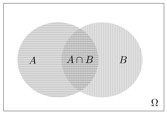
Figure 1.2.1: Two circular sets $A,B$, their intersection $A\cap B$ (gray area with horizontal and vertical lines), and their union $A\cup B$ (gray area with either horizontal or vertical lines or both). The set $\Omega\setminus (A\cup B)=(A\cup B)^c=A^c\cap B^c$ is represented by white color.
Definition 1.2.2
For a finite sample space $\Omega$, an event containing a single
element $E=\{\omega\}$, $\omega\in\Omega$ is called an elementary event.
If the sample space is finite $\Omega=\{\omega_1,\ldots,\omega_n\}$,
it is relatively straightforward to define probability functions by
defining the $n$ probabilities of the elementary events. More specifically, for a sample space with $n$ elements, suppose that we are given a set of $n$ non-negative numbers $\{p_{\omega}: \omega\in\Omega\}$ that sum to one. There exists then a unique probability function $\P$ over events such that $\P(\{\omega\})=p_{\omega}$. This probability is defined for arbitrary events through the finite additivity property
\[\P(E)=\sum_{\omega\in E} \P(\{\omega\})=\sum_{\omega\in E} p_{\omega}.\]
A similar argument holds for sample spaces that are countably infinite.
The R code below demonstrates such a probability function, defined on $\Omega=\{1,2,3,4\}$ using $p_1=1/2$, $p_2=1/4$, $p_3=p_4=1/8$.
Omega = c(1, 2, 3, 4)
p = c(1/2, 1/4, 1/8, 1/8)
sum(p)
A = c(1, 0, 0, 1)
sum(p[A == 1])