3.11. The t Distribution
A $t_{\nu}$ RV, where $\nu > 0$ is a parameter called the degrees of freedom, has the following pdf \begin{align*} f_X(x) &= \frac{\Gamma(\frac{\nu+1}{2})}{\sqrt{\nu\pi}\,\Gamma(\nu/2)} \left(1+\frac{x^2}{\nu}\right)^{-\frac{\nu+1}{2}}, \quad x\in\R, \nu>0. \end{align*}
It can be shown that if $Z\sim N(0,1), W\sim \chi^2_{\nu}$ are two independent RVs, then \[\frac{Z}{\sqrt{W/\nu}} \sim t_{\nu}.\]
The $t$ distribution with $\nu=1$ is called the Cauchy distribution. Its pdf is \[ f_X(x) = \frac{1}{\pi(1+x^2)}. \] The $t$ distribution with $\nu=2$ has the following pdf \[ f_X(x) = \frac{1}{(2+x^2)^{2/3}}.\] As $\nu$ increases, the polynomial decay becomes sharper. At the limit $\nu\to\infty$ the $t$ distribution pdf converges to the pdf of a $N(0,1)$ RV.
The main use of the $t$-distribution is in statistical tests and confidence intervals. In addition, it is also used to model heavy tailed distributions. A $t_{\nu}$-RV decays qualitatively slower than any Gaussian RV, regardless of the $\nu$ parameter. In fact, the decay of the $t_{\nu}$-RV pdf is so slow that for $\nu < 1$ the expectation does not exist (the integral diverges). Similarly, the variance of $t_{\nu}$ is $\infty$ for $1 < \nu\leq 2$ and is undefined for $\nu\leq 1$.
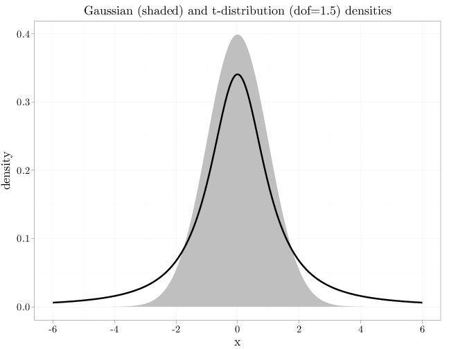
The R code below graphs the pdfs of a Gaussian and a $t$ RVs. Both have symmetric bell-shaped pdf, but the $t$ pdf decays more slowly and is sharper and the center.
x = seq(-6, 6, length.out = 200)
R = data.frame(density = dnorm(x, 0, 1))
R$tdensity = dt(x, 1.5)
R$x = x
P = ggplot(R, aes(x = x, y = density)) + geom_area(fill = I("grey")) +
    geom_line(aes(x = x, y = tdensity), xlab = "$x$",
        ylab = "$f_X(x)$", lwd = I(2))
P + opts(title = "Gaussian (shaded) and t-distribution (dof=1.5) densities")