Probability
The Analysis of Data, volume 1
Random Variables: Functions of a Random Variable
$
\def\P{\mathsf{P}}
\def\R{\mathbb{R}}
\def\defeq{\stackrel{\tiny\text{def}}{=}}
\def\c{\,|\,}
\def\bb{\boldsymbol}
\def\diag{\operatorname{\sf diag}}
$
2.2. Functions of a Random Variable
Definition 2.2.1.
Composing an RV $X:\Omega\to\R$ with $g:\R\to\R$ defines a new RV
$g\circ X:\Omega\to\R$, which we denote by $g(X)$. In other words, $g(X)(\omega)=g(X(\omega))$ (see Figure 2.2.1).
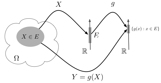
Figure 2.2.1: Given an RV $X$, the RV $Y=g(X)$ is a mapping from $\Omega$ to $\mathbb{R}$ realized by $\omega\mapsto g(X(\omega))$. Contrast this with Figure 2.1.1.
We can compute probabilities of events relating to $Y=g(X)$ through probabilities of events concerning $X$:
\begin{align} \tag{2.2.1}
\P(Y\in B) &= \P(\{\omega\in\Omega:Y(\omega)\in B\})\\ &=
\P(\{\omega\in\Omega:g(X(\omega))\in B\}) \nonumber \\
&=\P(\{\omega\in\Omega:X(\omega)\in g^{-1}(B)\}) \nonumber \\&= \P(X\in g^{-1}(B))\nonumber
\end{align}
where $g^{-1}(B)=\{r\in\R:g(r)\in B\}$. In other words, if we can compute quantities such as $\P(X\in A)$, we can also compute quantities such as $\P(g(X)\in B)$. This implies a relationship between the cdfs, pdfs, and pmfs of $X$ and $Y=g(X)$, on which we elaborate below.
Discrete $g(X)$
For a discrete RV $X$ and $Y=g(X)$, Equation (2.2.1) implies
\begin{align*}
p_Y(y)=\P(Y=y)=\P(g(X)=y)=\P(X\in g^{-1}(\{y\}))=\sum_{x:g(x)=y}p_X(x).
\end{align*}
In particular, if $g$ is one-to-one, then $p_Y(y)=p_X(x)$ for the $x$ satisfying
$g(x)=y$.
Example 2.2.1.
In the coin-toss experiment (Example 2.1.2), we computed that $p_X(0)=p_X(3)=1/8, p_X(1)=p_X(2)=3/8$ and $p_X(x)=0$ otherwise. The function $g(r)=r^2-2$ is one-to-one on the set $A$ for which $\P(X\in A)=1$ ($A=\{0,1,2,3\}$). We therefore have the following pmf of $Y=g(X)=X^2-2$
\[ p_Y(y) =
\begin{cases}
p_X(0)=1/8 & y=-2\\
p_X(1)=3/8 & y=-1\\
p_X(2)=3/8 & y=2\\
p_X(3)=1/8 & y=7\\
0 & \text{otherwise}
\end{cases}.
\]
By contrast, the function \[h(r)=\begin{cases} 0 & r < 3/2\\1 & r \geq 3/2\end{cases}\]
is not one-to-one on the set $A=\{0,1,2,3\}$, suggesting that more than one value of $x$ contributes to each value of $y$. Specifically, $h(0)=h(1)=0$ and $h(2)=h(3)=1$, implying that the pmf of the RV $Z=h(X)$ is
\[ p_Z(r) = \begin{cases}
p_X(0)+p_X(1)=1/8+3/8=1/2 & r=0\\
p_X(2)+p_X(3)=1/8+3/8=1/2 & r=1\\
0 & \text{otherwise}\end{cases}.
\]
Continuous $g(X)$
If $X$ is a continuous RV, $Y=g(X)$ can be discrete, continuous, or neither. If $Y$ is a discrete RV, its pmf can be determined by the formula
\[p_Y(y)=\int_{\{r:g(r)=y\}} f_X(r)dr.\]
Example 2.2.2.
In the dart-throwing experiment (Example 2.1.3), the RV $Y=g(R)$, where $g(r)=0$ if $r<0.1$
and $g(r)=1$ otherwise, is a discrete RV with
\[p_Y(y)=\begin{cases}
\P(g(R)=0)=\int_0^{0.1} 2r\,dr=0.01 & y=0\\
\int_{0.1}^1 2r\,dr=0.99 & y=1\\ 0 & \text{otherwise}
\end{cases}.\]
If $g(X)$ is continuous, then we can compute the density $f_{g(X)}$ in three ways.
- Compute the cdf $F_Y(y)$ for all $y\in\mathbb{R}$ using Equation (2.2.1)
\[ F_Y(y)=\P(Y\leq y)=\P(g(X)\leq y)\]
and proceed to compute the pdf $f_{g(X)}$ by differentiating $F_{g(X)}$.
- Compute the density of $Y=g(X)$ directly from $f_X$ when $g:\R\to\R$ is differentiable and one-to-one on the domain of $f_X$, using the change of variables technique (see Section F.2)
\begin{align} \tag{2.2.2}
f_{g(X)}(y)=\frac{1}{|g'(g^{-1}(y))|}f_X(g^{-1}(y)).
\end{align}
The requirement that $g$ be one-to-one is essential since otherwise the inverse function $g^{-1}$ fails to exist.
- Compare the moment generating function (defined in Section 2.4) of $Y$ to that of a known RV.
Example 2.2.3.
We can apply the first of the three techniques to the dart-throwing experiment (Example 2.1.3). The RV $Y=g(R)=R^2$ ($g(r)=r^2$) is a continuous RV with
\begin{align*}
F_Y(y) &=
\begin{cases} \P(R^2\leq y) = \P\left(\left\{\omega\in\Omega: R(\omega)\leq\sqrt{y}\right\}\right)=F_R(\sqrt{y})=\frac{\pi (\sqrt{y})^2}{\pi \cdot 1} & y\in (0,1)\\
0 & y < 0\\
1 & y \geq 1\end{cases}\\
f_Y(y) &= F_Y'(y)=\begin{cases} 1 & y\in (0,1)\\ 0 & \text{otherwise}\end{cases}.
\end{align*}
Since the function $g(r)=r^2$ is increasing and differentiable in $(0,1)$ and $\P(R\in (0,1))=1$, we can also use Equation (2.2.2)
\[f_Y(y)=\frac{1}{|g'(\sqrt{y})|} f_R(\sqrt{y})
=\frac{1}{2\sqrt{y}} 2\sqrt{y}=1 \]
for $0 < y < 1$ and 0 otherwise.
Example 2.2.4.
Let $X$ be a continuous RV with a cdf $F_X$ strictly increasing on the range of $X$. Using Equation (2.2.2) above, the RV $Y=F_X(X)$ has the pdf
\[ f_Y(y) = \frac{1}{f_X(F_X^{-1}(y))} f_X(F_X^{-1}(y))=\begin{cases}1 & y\in [0,1]\\ 0 &\text{otherwise}\end{cases}.\]
The second branch above ($y\not\in[0,1]$) follows since $F_X$ is not strictly monotonic increasing outside of $[0,1]$ and therefore Equation (2.2.2) does not apply outside of $[0,1]$. In that region we identify $\P(Y\leq a)$ for $a\not\in[0,1]$ is constant, implying that its derivative, the pdf, is zero.
The transformation $X\mapsto Y=F_X(X)$ maps a continuous RV $X$ into an RV $F_X(X)$ with a a pdf that is constant over $[0,1]$ and 0 elsewhere. This RV corresponds to the classical probability model on $(0,1)$ (see Section 1.4). We will encounter this RV again in the next chapter.
Note that the same reasoning does not hold when $X$ is discrete since in that case $F_X$ is not one-to-one and $F_X^{-1}$ does not exist.
Example 2.2.5.
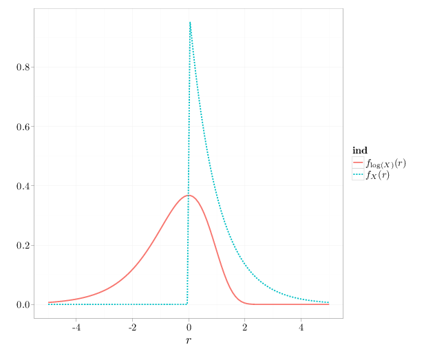
Consider an RV $X$ with $f_X(x)=\exp(-x)$ for $x\geq 0$ and 0 otherwise. Using Equation (2.2.2), the pdf of $Y=g(X)=\log(X)$ is
\begin{align*}
f_Y(y)=\frac{1}{|1/e^y|}\exp(-\exp(y))=\exp(y-\exp(y)).
\end{align*}
(Note that $g(x)=\log(x)$, $g^{-1}(y)=\exp(y)$, $g'(x)=1/x$.)
The following R code and graph contrasts the pdfs of $X$ and $Y=\log(X)$.
x = seq(-5, 5, length = 100)
Y1 = exp(-x)
Y1[x < 0] = 0
Y2 = exp(x - exp(x))
D = stack(list(`$f_X(r)$` = Y1, `$f_{\\log(X)}(r)$` = Y2))
D$x = x
qplot(x, values, xlab = "$r$", ylab = "", geom = "line",
    color = ind, lty = ind, data = D, size = I(1.5))
The calculation above shows that \[f_{g(X)}(r)\neq g\circ f_X(r)=g(f_X(r)).\] The right hand side above is often mistakenly taken to be the density of $g(X)$, but is in most cases not even a density function (for example in this example $g(f_X(r))$ would assume negative values).