3.5. The Negative Binomial Distribution
The negative binomial RV, $X\sim NB(r,\theta)$, where $r\in\mathbb{N}\cup\{0\}, \theta\in[0,1]$, is the number of successes in an infinite sequence of independent Bernoulli experiments before encountering $r$ failures.
The mass function of $X\sim NB(r,\theta)$ is \begin{align} p_X(x) = \begin{cases} \begin{pmatrix} x+r-1\\x \end{pmatrix} (1-\theta)^r \theta^x & x\in\mathbb{N}\cup\{0\}\\ 0 & \text{otherwise}\end{cases}. \end{align}
The above pmf can be derived by noting that there are $\begin{pmatrix} x+r-1\\x \end{pmatrix}$ arrangements of $r$ failures and $x$ successes with the last failure occurring at the end, and that each of the arrangements occur with probability $(1-\theta)^r \theta^x$.
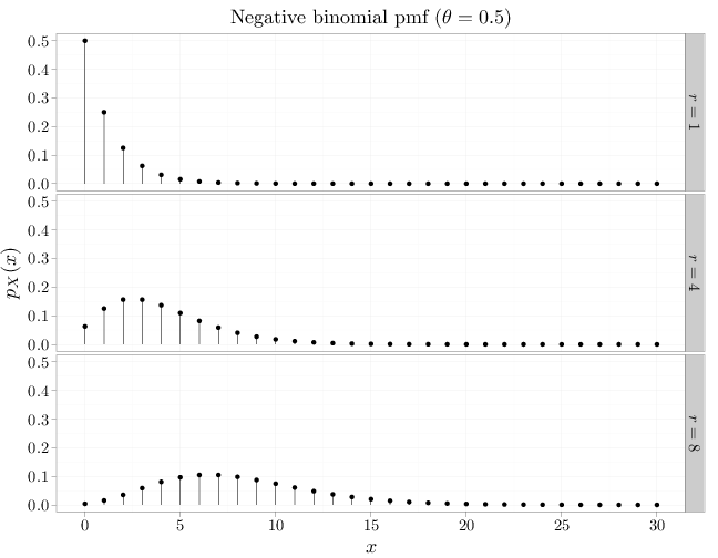
The R code below graphs the pmfs of multiple negative binomial RVs with different parameter values.
theta = 0.5
x = 0:30
D = stack(list(`$r=1$` = dnbinom(x, 1, theta), `$r=4$` = dnbinom(x,
    4, theta), `$r=8$` = dnbinom(x, 8, theta)))
names(D) = c("mass", "r")
D$x = x
qplot(x, mass, data = D, geom = "point", stat = "identity",
    facets = r ~ ., xlab = "$x$", ylab = "$p_X(x)$",
    main = "Negative binomial pmf ($\\theta=0.5$)") +
    geom_linerange(aes(x = x, ymin = 0, ymax = mass))
