3.1. The Bernoulli Trial Distribution
Below, we denote the distributions corresponding to the different random variables using abbreviations such as Ber or Bin. In cases where the distributions are parameterized, we attach the parameter or parameters to the abbreviation, for example $\text{Bin}(n,\theta)$. We use the notation $\sim$ to denote "distributed according to", for example $X\sim\text{Ber}(\theta)$ implies that the RV $X$ follows the $\text{Ber}(\theta)$ distribution.
The Bernoulli trial RV, $X\sim\text{Ber}(\theta)$, where $\theta\in[0,1]$, is characterized by the following pmf: \[p_X(x)=\begin{cases} \theta & x=1\\ 1-\theta & x=0\\0&\text{otherwise}\end{cases}, \qquad \theta\in [0,1].\] The Bernoulli trial RV may be used to characterize the probability that an experiment (or trial) that may either succeed, $X=1$, or fail, $X=0$, with probabilities $\theta$, $1-\theta$ respectively. A popular example of such an experiment is flipping a potentially biased coin, with success corresponding to heads and failure corresponding to tails.
The expectation and variance of $X\sim\text{Ber}(\theta)$ are: \begin{align*} \E(X)&=1\theta+0(1-\theta)=\theta\\ \Var(X)&=\E(X^2)-E^2(X)=1^2\theta+0^2(1-\theta)-\theta^2=\theta(1-\theta). \end{align*}
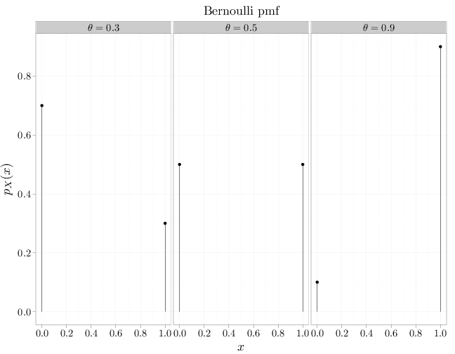
The R code below graphs the mass functions corresponding to three different $\theta$ parameters.
x = c(0, 1)
D = stack(list(`$\\theta=0.3$` = dbinom(x, 1, 0.3),
    `$\\theta=0.5$` = dbinom(x, 1, 0.5), `$\\theta=0.9$` = dbinom(x,
        1, 0.9)))
names(D) = c("mass", "theta")
D$x = x
qplot(x, mass, data = D, main = "Bernoulli pmf", geom = "point",
    stat = "identity", facets = . ~ theta, xlab = "$x$",
    ylab = "$p_X(x)$") + geom_linerange(aes(x = x,
    ymin = 0, ymax = mass))