3.9. The Gaussian Distribution
The Gaussian or normal RV, $X\sim N(\mu,\sigma^2)$, where $\mu\in\mathbb{R}, \sigma^2 > 0$, has the pdf \[f_X(x)=\frac{1}{\sqrt{2\pi\sigma^2}}\exp\left(-\frac{(x-\mu)^2}{2\sigma^2}\right).\] If $\mu=0,\sigma^2=1$, we refer to this RV as the standard normal or standard Gaussian RV. We sometimes attach the parameters $\mu,\sigma$ as subscripts, for example $f_{0,1}$ and $F_{0,1}$ denote the pdf and cdf of $X_{0,1}$, the standard normal RV. A common notation for $F_{0,1}(x)$ is $\Phi(x)$.
To verify that the pdf integrates to 1, we use the change of variable $(x-\mu)/\sigma \mapsto y$ to get \begin{align*} \int_{-\infty}^{\infty} \frac{1}{\sqrt{2\pi}\sigma} \exp\left(-\frac{(x-\mu)^2}{2\sigma^2}\right) dx &= \int_{-\infty}^{\infty} \frac{1}{\sqrt{2\pi}}\exp\left(-y^2/2\right) \, dy \\ &= \frac{1}{\sqrt{2\pi}} \sqrt{2\pi}=1 \end{align*} where the first equality follows from Example F.2.3 and the second from Example F.6.1.
Example F.2.3 (substitute $a=-\infty$ and $b=x$) shows the following relations between the cdfs and pdfs of the Gaussian distribution: \begin{align} \tag{*} F_{\mu,\sigma^2}(x) &= F_{0,1}\left(\frac{x-\mu}{\sigma}\right)=\Phi\left(\frac{x-\mu}{\sigma}\right),\\ f_{\mu,\sigma^2}(x) &= \frac{d}{d x} F_{\mu,\sigma^2}(x)=\frac{d}{dx} F_{0,1}\left(\frac{x-\mu}{\sigma}\right) = \frac{1}{\sigma} f_{0,1}\left(\frac{x-\mu}{\sigma}\right).\notag \end{align} (The last equality follows from the chain rule (Proposition D.1.3).)
Differentiating the mgf, we have for $X\sim N(\mu,\sigma^2)$, \begin{align*} \E(X) & = \psi'(0) = (\mu+\sigma^2 0)1=\mu\\ \Var(X) &= \E(X^2)-(\E (X))^2 = \psi''(0)-\mu^2= \sigma^2 1 + (\mu+0)^2 1 - \mu^2 = \sigma^2. \end{align*}
The Gaussian distribution is one of the most important distributions. The central limit theorem (see Section 8.9 for details) informally states that a sum of many independent random variables is approximately a Gaussian distribution. As a consequence, quantities that are sums of a large number of independent random factors are approximately Gaussian. Examples include performance measures like IQ test results and physiological measurements like height.
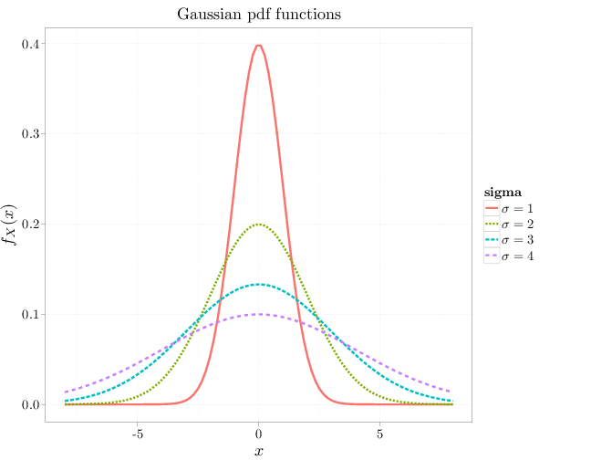
The R code below graphs the pdf of the Gaussian distribution for different values of $\sigma$ and $\mu$.
x = seq(-8, 8, length.out = 100)
gf = function(x, s) exp(-x^2/(2 * s^2))/(sqrt(2 * pi) *
    s)
R = stack(list(`$\\sigma=1$` = gf(x, 1), `$\\sigma=2$` = gf(x,
    2), `$\\sigma=3$` = gf(x, 3), `$\\sigma=4$` = gf(x,
    4)))
# below, x is recycled four times
names(R) = c("y", "sigma")
R$x = x
qplot(x, y, color = sigma, main = "Gaussian pdf functions",
    lty = sigma, lwd = I(2), geom = "line", xlab = "$x$",
    ylab = "$f_X(x)$", data = R)
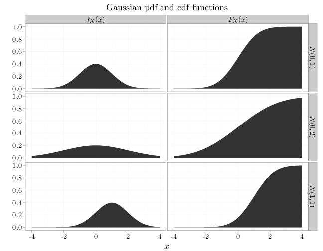
x = seq(-4, 4, length = 100)
y1 = dnorm(x, 0, 1)
y2 = dnorm(x, 1, 1)
y3 = dnorm(x, 0, 2)
y4 = pnorm(x, 0, 1)
y5 = pnorm(x, 1, 1)
y6 = pnorm(x, 0, 2)
D = data.frame(probability = c(y1, y2, y3, y4, y5,
    y6))
D$x = x
D$parameter[1:100] = "$N(0,1)$"
D$parameter[301:400] = "$N(0,1)$"
D$parameter[101:200] = "$N(1,1)$"
D$parameter[401:500] = "$N(1,1)$"
D$parameter[201:300] = "$N(0,2)$"
D$parameter[501:600] = "$N(0,2)$"
D$type[1:300] = "$f_X(x)$"
D$type[301:600] = "$F_X(x)$"
qplot(x, probability, data = D, main = "Gaussian pdf and cdf functions",
    geom = "area", facets = parameter ~ type, xlab = "$x$",
    ylab = "")