Important Random Vectors: The Dirichlet Random Vector

Probability

The Analysis of Data, volume 1

0
- Front Matter
- 0.1: Contents
- 0.2: Preface
1
2
- Random Variables
- 2.1: Basic Definitions
- 2.2: Functions of RVs
- 2.3: Expectation and Variance
- 2.4: Moments and MGF
- 2.5: RVs and Measure Theory
- 2.6: Notes
- 2.7: Exercises
3
4
5
- Important Vectors
- 5.1: Multinomial Vectors
- 5.2: Gaussian Vectors
- 5.3: Dirichlet Vectors
- 5.4: Mixture Vectors
- 5.5: Exponential Family
- 5.6: Notes
- 5.7: Exercises
6
- Random Processes
- 6.1: Basic Definitions
- 6.2: Marginals
- 6.3: Moments
- 6.4: Random Walk
- 6.5: Processes and Measure
- 6.6: Borell-Cantelli and Zero-One
- 6.7: Notes
- 6.8: Exercises
7
- Important RPs
- 7.1: Markov Chains
- 7.2: Poisson Process
- 7.3: Gaussian Process
- 7.4: Notes
- 7.5: Exercises
8
A
- Set Theory
- A.1: Basic Definition
- A.2: Functions
- A.3: Cardinality
- A.4: Limits of Sets
- A.5: Notes
- A.6: Exercises
B
- Metric Spaces
- B.1: Basic Definitions
- B.2: Limits
- B.3: Continuity
- B.4: Euclidean Space
- B.5: Growth of Functions
- B.6: Notes
- B.7: Exercises
C
- Linear Algebra
- C.1: Basic Definitions
- C.2: Rank
- C.3: Eigenvalues and Determinant
- C.4: Semidefinite Matrices
- C.5: SVD
- C.6: Notes
- C.7: Exercises
D
- Differentiation
- D.1: Scalar Differentiation
- D.2: Power and Taylor Series
- D.3: Notes
- D.4: Exercises
E
- Measure Theory
- E.1: Sigma Algebras
- E.2: Measure Function
- E.3: Extension Theorem
- E.4: Independence
- E.5: Important Measures
- E.6: Measurable Functions
- E.7: Notes
F

$\def\P{\mathsf{\sf P}} \def\E{\mathsf{\sf E}} \def\Var{\mathsf{\sf Var}} \def\Cov{\mathsf{\sf Cov}} \def\std{\mathsf{\sf std}} \def\Cor{\mathsf{\sf Cor}} \def\R{\mathbb{R}} \def\c{\,|\,} \def\bb{\boldsymbol} \def\diag{\mathsf{\sf diag}} \def\defeq{\stackrel{\tiny\text{def}}{=}}$

5.3. The Dirichlet Random Vector

Definition 5.3.1. The Dirichlet random vector

$\bb X\sim\text{Dir}(\bb\alpha)$ , where

$\alpha\in\mathbb{R}^k$ with

$\alpha_i\geq 0$ for all

$i=1,\ldots,k$ , is a continuous random vector, defined by

$\begin{align*} X_i = \frac{W_i}{\sum_{i=1}^k W_i}, \quad i=1,\ldots,k, \end{align*}$ where

$W_i\sim\text{Gam}(\alpha_i,1)$ ,

$i=1,\ldots,k$ are independent Gamma RVs (see Section 3.10).

Proposition 5.3.1. The Dirichlet random vector

$\bb X\sim\text{Dir}(\bb\alpha)$ has the following pdf

$\begin{align*} f_{\bb X}(\bb x) =\frac{\Gamma\left(\sum_{i=1}^k\alpha_i\right)}{\prod_{i=1}^k \Gamma(\alpha_i)} \,\,\prod_{i=1}^k x_i^{\alpha_i-1} \end{align*}$ if

$\bb x\in\mathbb{P}_k$ and

$f_{\bb X}(\bb x)=0$ otherwise.

Proof. We can obtain the pdf by applying the change of variable technique to the following pdf of the random vector

$\bb W$

$f_{\bb W}(\bb w) = \prod_{i=1}^k e^{-w_i} w_i^{\alpha_i-1} / \Gamma(\alpha_i),$ and the invertible transformation

$\bb W\mapsto (X_1,\ldots,X_{k-1},Z)$ where

$X_i = \frac{W_i}{\sum_{i=1}^k W_i}$ and

$Z=\sum_{i=1}^k W_i$ . We can express the transformation as

$W_i=X_i Z$ for

$i=1,\ldots,k-1$ and

$W_k=Z X_k=Z(1-X_1-\cdots- X_{k-1})$ . It follows that the Jacobian of the transformation is the following matrix

$\begin{align*} J=\begin{pmatrix} Z & 0 & \cdots & X_1\\ 0 & Z & \cdots & X_2\\ \vdots & \vdots & \ddots & \vdots\\ -Z & \cdots & -Z & X_k \end{pmatrix}. \end{align*}$

To use the change of variables technique, we need to compute the determinant of the matrix above. Recalling that adding one of the rows of the matrix to another row does not change the determinant, we can add the first $k-1$ rows to the last row, and then compute the determinant of the resulting matrix. That matrix is an upper diagonal matrix (all elements below the diagonal are zero) with diagonal elements $Z, Z, \cdots, Z, 1$ . Since the determinant of an upper diagonal matrix is the product of the diagonal terms (all other terms in the product defining the determinant expression zero out), the determinant is $Z^{k-1}$ . It follows that the pdf of the transformed variables $(X_1,\ldots,X_{k-1},Z)$ is $\begin{align*} f_{X_1,\ldots,X_{k-1},Z}(x_1,\ldots,x_{k-1},z) &= z^{k-1} \prod_{i=1}^k e^{-x_i z} (x_i z)^{\alpha_i-1} / \Gamma(\alpha_i)\\ &= z^{\sum \alpha_i-1} e^{-1\cdot z} \prod_{i=1}^k x_i^{\alpha_i-1} / \Gamma(\alpha_i). \end{align*}$

We integrate the above expression with respect to $z$ in order to obtain the pdf of $X_1,\ldots,X_{k-1}$ . $\begin{align*} f_{X_1,\ldots,X_{k-1}}(x_1,\ldots,x_{k-1}) &= \prod_{i=1}^k x_i^{\alpha_i-1} / \Gamma(\alpha_i) \cdot \int_0^{\infty} z^{\sum \alpha_i-1} e^{-1\cdot z}\,dz\\ &= \prod_{i=1}^k x_i^{\alpha_i-1} / \Gamma(\alpha_i) \cdot \Gamma\left(\sum_{i=1}^k\alpha_i \right) \end{align*}$ where the last equation follows from the fact that Gamma pdf integrates to one (see Section 3.10). Since $\sum_{i=1}^k X_i=1$ , the RV $X_k$ must equal $1-\sum_{i=1}^{k-1}X_i$ . The pdf above therefore remains the same if we add the RV $X_k$ taking value $1-\sum_{i=1}^{k-1}X_i$ (the pdf becomes zero for all other values of $X_k$ ).

Recall that the simplex $\mathbb{P}_k$ represents the set of all probability functions on a sample space $\Omega$ of size $k$ . The Dirichlet distribution may thus be viewed as a distribution over distributions over a finite sample space.

Proposition 5.3.2. Let

$W_i\sim\text{Gam}(\alpha_i,1)$ ,

$i=1,\ldots,k$ be independent Gamma RVs. The random vector

$(X_1, \ldots,X_{k-1})$ , where

$X_i = W_i/\sum_{i=1}^k W_i$ for

$i=1,\ldots,k-2$ and

$X_{k-1}=(W_{k-1}+W_k)/\sum_{i=1}^k W_i$ is a Dirichlet random vector with parameter

$(\alpha_1,\ldots,\alpha_{k-2},\alpha_{k-1}+\alpha_k)$ .

Proof. Recall from Section 3.10 that a sum of independent Gamma RVs with the same second parameter is a Gamma RV whose parameter is the sum of the corresponding parameters. The rest of the proof follows from the definition of the Dirichlet distribution above.

It is straightforward to generalize the proposition above and show that whenever we aggregate some of the Gamma $W_i$ RVs in categories, and then form the normalization construction that defines the Dirichlet random vector, we obtain a Dirichlet random vector with a parameter vector that is similarly aggregated.

Proposition 5.3.3. Let

$\bb X$ be a Dirichlet random vector with parameter vector

$\bb \alpha$ . The marginal distribution of

$X_i$ is

$\text{Beta}(\alpha_i,\sum_{j=1}^k \alpha_j - \alpha_i)$ , and we have

$\begin{align*} \E(X_i) &= \frac{\alpha_i}{\sum_{j=1}^k \alpha_j}\\ \Var(X_i) &= \frac{\alpha_i(\sum_{j=1}^k \alpha_j-\alpha_i)}{(\sum_{j=1}^k \alpha_j)^3-(\sum_{j=1}^k \alpha_j)^2}. \end{align*}$

Proof. Let

$W_i\sim\text{Gam}(\alpha_i,1)$ ,

$i=1,\ldots,k$ be the Gamma RVs underlying the Dirichlet construction of

$\bb X$ . The proposition states that the Dirichlet construction corresponding to the Gamma RVs

$W_i$ and

$\sum_{j:j\neq i} W_j$ results in a random vector

$(X_i, 1-X_i)$ that have a Dirichlet distribution with a parameter vector

$(\alpha_i,\sum_{j:j\neq i}\alpha_j)$ . Comparing the pdf of

$\text{Dir}(\alpha_i,\sum_{j:j\neq i}\alpha_j)$ to the beta distribution pdf, and noting that the distribution of

$X_i$ is directly obtained from the distribution of

$(X_i, 1-X_i)$ (the second RV is a function of the first and therefore it is a deterministic quantity) concludes the first part of the proof. The second part of the proof follows from the derivations of the expectation and variance of the beta distribution (see Section 3.12).

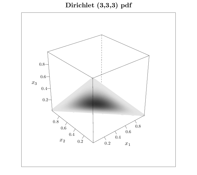
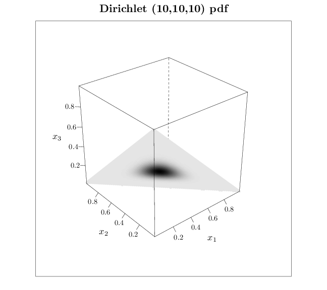
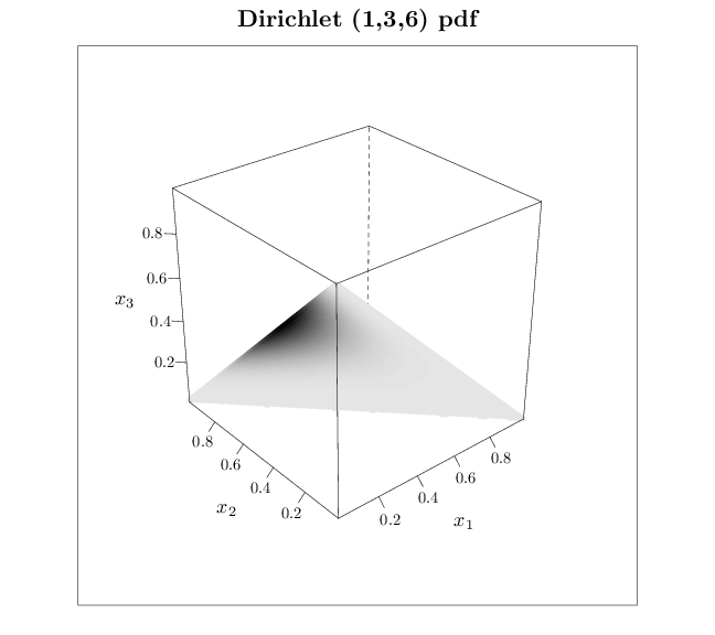
The R code below graphs the pdf of several Dirichlet distributions. Dark shades correspond to high probability and light shades correspond to low probabilities. Note that the pdf assigns non-zero values only to the simplex $\mathbb{P}_k$ (in this case $k=2$ ).

library(MCMCpack)
trellis.par.set(list(fontsize = list(text = 18)))
R = expand.grid(seq(0.001, 0.999, length.out = 80),
    seq(0.001, 0.999, length.out = 80))
R[, 3] = 1 - R[, 1] - R[, 2]
names(R) = c("x1", "x2", "x3")
R = R[R[, 3] > 0, ]
for (i in 1:nrow(R)) R$p[i] = ddirichlet(R[i, 1:3],
    alpha = c(3, 3, 3))
cloud(x3 ~ x1 * x2, data = R, col = gray(1 - R$p/(max(R$p) +
    3) - 0.1), pch = 16, cex = 1, main = "Dirichlet (3,3,3) pdf ",
    scales = list(arrows = FALSE), xlab = "$x_1$",
    ylab = "$x_2$", zlab = "$x_3$")

for (i in 1:nrow(R)) R$p[i] = ddirichlet(R[i, 1:3],
    alpha = c(10, 10, 10))
cloud(x3 ~ x1 * x2, data = R, col = gray(1 - R$p/(max(R$p) +
    3) - 0.1), pch = 16, cex = 0.8, main = "Dirichlet (10,10,10) pdf ",
    scales = list(arrows = FALSE), xlab = "$x_1$",
    ylab = "$x_2$", zlab = "$x_3$")

for (i in 1:nrow(R)) R$p[i] = ddirichlet(R[i, 1:3],
    alpha = c(1, 3, 6))
cloud(x3 ~ x1 * x2, data = R, col = gray(1 - R$p/(max(R$p) +
    3) - 0.1), pch = 16, cex = 0.8, main = "Dirichlet (1,3,6) pdf",
    scales = list(arrows = FALSE), xlab = "$x_1$",
    ylab = "$x_2$", zlab = "$x_3$")