3.12. The Beta Distribution
The beta RV $\text{Beta}(\alpha,\beta)$, where $\alpha,\beta > 0$, has the following pdf \begin{align*} f_X(x) &= \begin{cases} \frac{1}{B(\alpha,\beta)} x^{\alpha-1}(1-x)^{\beta-1} & x\in[0,1]\\ 0 & x\not\in[0,1] \end{cases}, \end{align*} where \begin{align*} B(\alpha,\beta) = \frac{\Gamma(\alpha)\Gamma(\beta)}{\Gamma(\alpha+\beta)} \end{align*} is the beta function.
Example F.6.1 verifies that the pdf integrates to 1 and can be used to compute the expectation and other moments \begin{align*} \E(X^k) &= \frac{1}{B(\alpha,\beta)} \int_0^{\infty} x^{\alpha+k-1}(1-x)^{\beta-1}\,dx = \frac{B(\alpha+k,\beta)}{B(\alpha,\beta)}\\ \E(X) &= \frac{B(\alpha+1,\beta)}{B(\alpha,\beta)} = \frac{\alpha}{\alpha+\beta}. \end{align*}
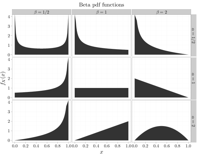
If $\alpha=\beta=1$ the beta distribution reduces to the uniform distribution over $[0,1]$. For other values of $\alpha,\beta$, however, we get a different behavior. When $\alpha < 1,\beta < 1$ the pdf has a U-shape over $[0,1]$. When $\alpha < 1$ and $\beta\geq 1$ the pdf is strictly decreasing. When $\alpha\geq 1$ and $\beta < 1$ the pdf is strictly increasing. Finally, when $\alpha>1$ and $\beta>1$ the pdf is unimodal, with a local maximum in $(0,1)$. If $\alpha=\beta$ the pdf is symmetric around 1/2 and if $\alpha\neq \beta$ the pdf is asymmetric around 1/2. The R code below graphs pdf functions of the beta distribution.
x = seq(0, 1, length = 100)
y1 = dbeta(x, 1/2, 1/2)
y2 = dbeta(x, 1/2, 1)
y3 = dbeta(x, 1/2, 2)
y4 = dbeta(x, 1, 1/2)
y5 = dbeta(x, 1, 1)
y6 = dbeta(x, 1, 2)
y7 = dbeta(x, 2, 1/2)
y8 = dbeta(x, 2, 1)
y9 = dbeta(x, 2, 2)
D = data.frame(probability = c(y1, y2, y3, y4, y5,
    y6, y7, y8, y9))
D$x = x
D$alpha[1:300] = "$\\alpha=1/2$"
D$alpha[301:600] = "$\\alpha=1$"
D$alpha[601:900] = "$\\alpha=2$"
D$beta[1:100] = "$\\beta=1/2$"
D$beta[101:200] = "$\\beta=1$"
D$beta[201:300] = "$\\beta=2$"
D$beta[301:400] = "$\\beta=1/2$"
D$beta[401:500] = "$\\beta=1$"
D$beta[501:600] = "$\\beta=2$"
D$beta[601:700] = "$\\beta=1/2$"
D$beta[701:800] = "$\\beta=1$"
D$beta[801:900] = "$\\beta=2$"
qplot(x, probability, main = "Beta pdf functions",
    data = D, geom = "area", facets = alpha ~ beta,
    xlab = "$x$", ylab = "$f_X(x)$", ) + scale_y_continuous(limits = c(0,
    4))