$
\def\P{\mathsf{P}}
\def\R{\mathbb{R}}
\def\defeq{\stackrel{\tiny\text{def}}{=}}
\def\c{\,|\,}
\def\bb{\boldsymbol}
\def\diag{\operatorname{\sf diag}}
$
In this chapter we continue studying probability theory, covering random variables and their associated functions: cumulative distribution functions, probability mass functions, and probability density functions.
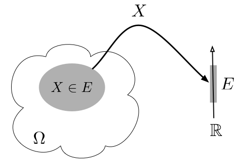
Figure 2.2.1: A random variable $X$ is a mapping from $\Omega$ to $\mathbb{R}$. The set $X\in E$ or $\{X\in E\}$, $E\subset \mathbb{R}$, corresponds to $\{\omega\in\Omega: X(\omega)\in E\}$ and $\P(X\in E)=\P(\{\omega\in\Omega: X(\omega)\in E\})$.
An RV $X:\Omega\to \R$ defines a new probability function $\P'$ on a new sample space $\Omega'=\mathbb{R}$:
\begin{align} \tag{*}
\P'(E) = \P(X\in E), \qquad E\subset \mathbb{R}=\Omega'.
\end{align}
Verifying that $\P'$ satisfies the three probability axioms is straightforward. We can often leverage the conceptually simpler $(\R,\P')$ in computing probabilities $\P(A)$ of events $A=\{X\in E\}$, ignoring $(\Omega,\P)$.
Example 2.1.1.
In Example 1.3.1 (throwing two fair dice, $\Omega=\{\omega=(a,b):a\in\{1,\ldots,6\},b\in\{1,\ldots,6\}\}$, and $\P(A)=|A|/36$), the RV $X(a,b)=a+b$ (sum of the faces of the two dice) exhibits the following events and their associated probabilities.
\begin{align*}
\{X=3\}&=\{(1,2),(2,1)\}, & \P(\{X=3\})&=2/36\\
\{X=4\}&=\{(2,2),(3,1),(1,3)\},& \P(\{X=4\})&= 3/36\\
\{X < 3\}&=\{(1,1)\},& \P(\{X < 3\})&=1/36\\
\{X < 2\}&=\emptyset,& \P(\{X < 2\})&=0.
\end{align*}
Example 2.1.2.
In Example 1.1.1 (tossing three fair coins), the RV $X$ counting the number of heads gives the following events and their associated probabilities.
\begin{align*}
\P(X=0)&=\P(\{\omega\in\Omega:X(\omega)=0\})=\P(\{TTT\})=0.5^3=1/8\\
\P(X=1)&=\P(\{\omega\in\Omega:X(\omega)=1\})=\P(\{HTT,THT,TTH\})=3\cdot 0.5^3=3/8\\
\P(X=2)&=\P(\{\omega\in\Omega:X(\omega)=2\})=\P(\{HHT,HHT,HTH\})=3\cdot 0.5^3=3/8\\
\P(X=3)&=\P(\{\omega\in\Omega:X(\omega)=3\})=\P(\{HHH\})=0.5^3=1/8.
\end{align*}
Definition 2.1.2.
A random variable $X$ is discrete if $\P(X\in K)=1$ for some finite or countably infinite set $K\subset\R$. A random variable $X$ is continuous if $\P(X=x)=0$ for all $x\in\mathbb{R}$.
An RV can be discrete, continuous, or neither. If $\{X(\omega):\omega\in\Omega\}$ is finite or countably infinite, $X$ is discrete. This happens in particular if $\Omega$ is finite or countably infinite.
Example 2.1.3.
In the dart throwing experiment of Example 1.1.2, the sample space is $\Omega=\{(x,y):\sqrt{x^2+y^2}<1\}$. The RV $Z$, which is 1 for a bullseye and 0 otherwise, is discrete since $\P(Z\in\{0,1\})=1$. The RV $R$, defined as $R(x,y)=\sqrt{x^2+y^2}$, represents the distance of between the dart position and the origin. Since the 2-D area of a circle $\{R=r\}=\{(x,y):x,y\in\mathbb{R}, \sqrt{x^2+y^2}=r\}$ is zero, we have for all $r$, $\P(R=r)=\text{2D-area}(\{R=r\})/(\pi 1^2)=0$ (under the classical model), implying that $R$ is a continuous RV.
We also have
\begin{align*}
\P(R < r) &= \P\left(\left\{(x,y):x,y\in\mathbb{R}, \sqrt{x^2+y^2} < r\right\}\right) = \frac{\pi r^2}{\pi 1^2}=r^2 \\
\P(0.2 < R < 0.5) &= \P\left(\left\{(x,y):x,y\in\mathbb{R}, 0.2 < \sqrt{x^2+y^2} < 0.5\right\}\right)\\ &=\frac{\pi (0.5^2-0.2^2)}{\pi 1^2}.
\end{align*}
Definition 2.1.3.
We define the cumulative distribution function (cdf) with respect to an RV $X$ to be
$F_X:\mathbb{R}\to\mathbb{R}$ given by $F_X(x)=\P(X\leq x)$.
Definition 2.1.4.
Given a discrete RV $X$, we define the associated probability mass function (pmf) $p_X:\mathbb{R}\to\mathbb{R}$ to be $p_X(x)=\P(X=x)$.
Definition 2.1.5.
Given a continuous RV $X$, we define the associated probability density function (pdf)
$f_X:\mathbb{R}\to\mathbb{R}$ as the derivative of the cdf $f_X=F_X'$ where it exists, and 0 elsewhere.
The cdf is useful for both discrete and continuous RVs, the pmf is useful for discrete RVs only, and the pdf is useful for continuous RVs only. Notice that in each of the three functions above, we denote the applicable RV with an uppercase subscript and the function argument with a lowercase letter, and the two usually correspond (for example, $p_X(x)=\P(X=x)$).
We have the following relationship between the cdf and the pdf
\begin{align*}
f_X(r)&= \begin{cases} F_X'(r)& F_X'(r)\text{ exists}\\ 0 & \text{otherwise}\end{cases} \\
F_X(x)&=\int_{-\infty}^x f_X(r)\,dr.
\end{align*}
where the first equation follows from the definition of a pdf and the second line follows from the fundamental theorem of calculus (see Chapter E).
Example 2.1.4.
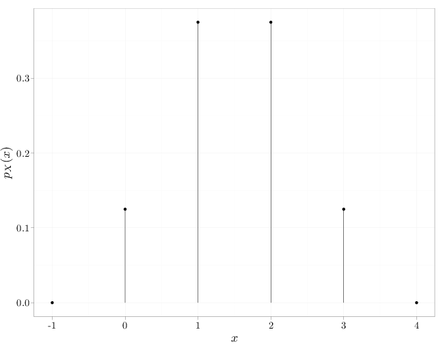
In the coin-tossing experiment (Example 2.1.2), we have
\begin{align*}
p_X(x)=\P(X=x)=\begin{cases} 1/8 & x=0 \\ 3/8 & x=1 \\ 3/8 & x=2\\
1/8 & x=3 \\ 0 & \text{else}
\end{cases} \qquad
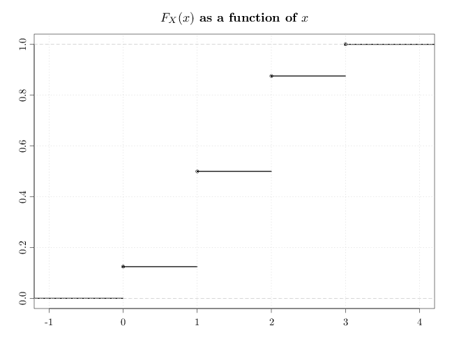
F_X(x)=\P(X\leq x)=\begin{cases} 0 & x < 0 \\ 1/8 & 0\leq x < 1 \\ 1/2 & 1\leq x < 2\\
7/8 & 2\leq x < 3 \\ 1 & 3 \leq x
\end{cases}.
\end{align*}
The following R code illustrates these pmf and cdf functions.
D = data.frame(x = c(-1, 0, 1, 2, 3, 4), y = c(0, 1/8,
    3/8, 3/8, 1/8, 0))
qplot(x, y, data = D, xlab = "$x$", ylab = "$p_X(x)$") +
    geom_linerange(aes(x = x, ymin = 0, ymax = y))
par(cex.main = 1.5, cex.axis = 1.2, cex.lab = 2)
plot(ecdf(c(0, 1, 1, 1, 2, 2, 2, 3)), verticals = FALSE,
    lwd = 3, main = "$F_X(x)$ as a function of $x$",
    xlab = "", ylab = "")
grid()
In the previous figure, the filled circles above clarify the value of $F_X$ at the discontinuity points above, for example $F_X(3)=1$. Note how the $F_X$ above is monotonic increasing from 0 to 1, and is continuous from the right, but not continuous from the left.
Example 2.1.5.
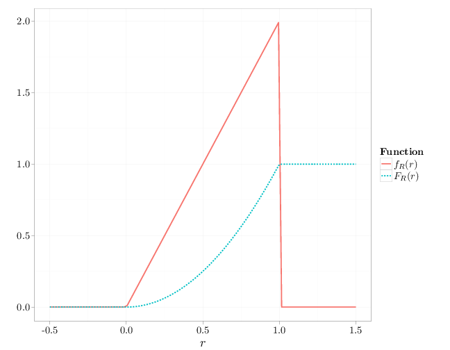
In the dart-throwing experiment (Example 2.1.3), we have
\begin{align*}
F_R(r)&=\P(R\leq r)=\begin{cases} 0 & r < 0 \\
\pi r^2 / (\pi 1^2)=r^2 & 0\leq r < 1\\
1 & 1\leq r
\end{cases}, \\
f_R(r)&=\frac{dF_R(r)}{dr}=\begin{cases} 0 & r<0 \\
2r & 0\leq r <1\\
0 & 1\leq r
\end{cases}.
\end{align*}
The following R code illustrates these pdf and cdf functions.
x = seq(-0.5, 1.5, length = 100)
y = x^2
y[x < 0] = 0
y[x > 1] = 1
z = 2 * x
z[x < 0] = 0
z[x > 1] = 0
D = stack(list(`$f_R(r)$` = z, `$F_R(r)$` = y))
names(D) = c("probability", "Function")
D$x = x
qplot(x, y = probability, geom = "line", xlab = "$r$",
    ylab = "", lty = Function, color = Function, data = D,
    size = I(1.5))
Proposition 2.1.1.
The pmf $p_X$ of a discrete RV satisfies
- $p_X(x)\geq 0$
- The set $\{x\in\mathbb{R}:p_X(x)\neq 0\}$ is finite or countably infinite
- $1=\sum_x p_X(x)$
- $\P(A)=\sum_{x\in A} p_X(x)$,
where the summations above contain only the finite or countably infinite number of terms for which $p_X$ is nonzero. Conversely, a function $p_X$ that satisfies the above properties is a valid pmf for some discrete RV.
Proof.
Statement (1) follows from the nonnegativity of $\P$ and (2) follows from the definition of a discrete RV. Statements (3) and (4) follow from (2) and the third axiom of probability functions. The converse statement holds since the probability $\P$ defined in (4) satisfies the probability axioms.
Lemma 2.1.1 (Continuity of the Probability Function). Let $A_n, n\in\mathbb{N}$ be a sequence of monotonic sets with a limit $A$. That is, either $A_1\subset A_2\subset A_3\subset \cdots$ with $A=\cup_n A_n$ or $\cdots\subset A_3\subset A_2\subset A_1$ with $A =\cap_n A_n$. Then $\lim_{n\to\infty} \P(A_n)=\P(A)$.
Proof*.
The result follows directly from the the continuity of measure proposition in Section E.2.
Proposition 2.1.2.
Denoting the left and right hand limits of $F_X$ by $F_X(a^-)=\lim_{x\to a^-} F_X(x)$ and $F_X(a^+)=\lim_{x\to a^+} F_X(x)$, respectively (see Definition B.2.11), we have
- $F_X(a^-)=\P(X < a)$,
- $F_X$ is monotonically increasing: if $a < b$, $F_X(a)\leq
F_X(b)$,
- $0=\lim_{a\to-\infty} F_X(a) < \lim_{a\to\infty} F_X(a)=1$, and
- $F_X$ is continuous from the right; that is for all $a\in\R$, $F_X(a)=F_X(a^+)$.
A function satisfying (2), (3), and (4) above is a cdf for some RV $X$.
Proof.
Statement (2) follows since $A\subset B$ implies that $\P(A)\leq \P(B)$. Statements (1), (3), (4) follow Lemma 2.1.1:
\begin{align*}
F_X(a^-) &= \lim_{n\to\infty} \P'((-\infty,a-1/n]) =
\P'( \cup_{n\in\mathbb{N}}(-\infty,a-1/n])=\P'((-\infty,a))\\
\lim_{n\to\infty} \P'((-\infty,-n]) &= \P'(\cap_{n\in\mathbb{N}}(-\infty,-n])=\P'(\emptyset)=0\\
\lim_{n\to\infty} \P'((-\infty,n]) &= \P'(\cup_{n\in\mathbb{N}}(-\infty,n])=\P'(\R)=1\\
\P'((-\infty,a])&=\P'(\cap_n (-\infty,a+1/n])=\lim_{n\to\infty} \P'((-\infty,a+1/n])=F_X(a^+).
\end{align*}
We can infer the converse since a function satisfying (2), (3), and (4) defines a unique probability measure on $\R$, as described and proved in Section E.5.
Corollary 2.1.1.
For all RV $X$ and $a < b$,
\begin{align*}
\P(a < X\leq b)&=F_X(b)-F_X(a)\\
\P(a\leq X\leq b)&=F_X(b)-F_X(a^-)\\
\P(a < X < b)&=F_X(b^-)-F_X(a) \\
\P(a\leq X < b)&=F_X(b^-)-F_X(a^-)\\
\P(X=x)&=F_X(x)-F_X(x^-).
\end{align*}
Proof.
These statements follow directly from the previous proposition.
Corollary 2.1.2.
The function $F_X$ is continuous if and only if $X$ is a continuous RV. In this case, \[F_X(a^-) = F_X(a) = F_X(a^+).\]
Proof.
An RV $X$ is continuous if and only if $0=\P(X=x)=F_X(x)-F_X(x^-)$ for all $x\in\R$, or in other words, the cdf is continuous from the left. Since the cdf is always continuous from the right, the continuity of $X$ is equivalent to the continuity of $F_X$.
Definition 2.1.6.
The quantile function associated with an RV $X$ is \[Q_X(r)=\inf\{x:F_X(x)=r\}.\]
The reason for the infimum in the definition above is that $F_X$ may not be a one-to-one function, and there may be multiple values $x$ for which $F_X(x)=r$. Recall that for a continuous $X$, the cdf $F_X$ is continuous and monotonic increasing from 0 at $-\infty$ to 1 at $\infty$ (see Definition B.2.5). If the cdf is strictly monotonically increasing (see Definition B.2.5), $F_X$ is one-to-one and hence invertible and
$Q_X(r)=F_X^{-1}(r)$. The value, $Q_X(1/2)$, at which 50% of the probability mass lies above and 50% of the probability mass lie below is called the median.
Proposition 2.1.3.
Let $X$ be a continuous RV. Then
- $f_X$ is a nonnegative function, and
- $\int_{\R} f_X(x)dx=1$.
A piecewise continuous function $f_X$ satisfying the above properties is a valid pdf for some continuous RV.
Proof.
Statement (1) follows from the fact that the pdf is a derivative of a monotonic increasing function (the cdf). Statement (2) follows from
\begin{align*}
\int_{-\infty}^{\infty}
f_X(x)dx &= \lim_{n\to\infty} \int_{-n}^n f_X(x)dx = \lim_{n\to\infty}
\P(-n\leq X \leq n) \\ &= \lim_{n\to\infty}(F_X(n)-F_X(-n)) = 1-0.
\end{align*}
The converse follows from the existence of a cdf via
\[F_X(x)=\int_{-\infty}^x f_X(r)\,dr\] (see the fundamental theorem of calculus in Chapter E) and the converse part of Proposition 2.1.2.
Since the pdf is the derivative of the cdf we have
\[f_X(x)=\lim_{\Delta\to 0}\frac{F_X(x+\Delta)-F_X(x)}{\Delta}.\] This implies that for a small positive $\Delta$
\begin{align*}
f_X(x) &\approx \frac{\P(x < X < x+\Delta)}{\Delta}, \quad\text{or}\\
f_X(x) \Delta &\approx \P(x < X < x+\Delta).
\end{align*}
The above derivations shows that $f_X(x)\Delta$ is approximately the probability that $X$ lies within an interval of width $\Delta$ around $x$.
Proposition 2.1.4.
\begin{align} \P(X\in A)=\begin{cases}\sum_{x\in A}p_X(x) &
X \text{ is discrete}\\ \int_A f_X(x)dx & X \text{ is continuous}
\end{cases}.\end{align}
Proof.
In the discrete case,
\[\P(X\in A)=\P(\cup_{x\in A} \{X=x\}) =
\sum_{x\in A} \P(X=x)=\sum_{x\in A} p_X(x).\]
The continuous case follows from the fact that the pdf is the derivative of the cdf and the relationship between a derivative and the definite integral (see the fundamental theorem of calculus in Chapter E).
Example 2.1.6.
In the coin-toss experiment (Example 2.1.2), we computed the pmf of X to be $p_X(0)=1/8, p_X(1)=3/8, p_X(2)=3/8, p_X(3)=1/8$, so indeed $\sum_{x\in X}p_X(x)=1$. Using the proposition above, we have \[\P(X>0)=\sum_{x\in \{1,2,\ldots\}}p_X(x)=p_X(1)+p_X(2)+p_X(3)=7/8.\]
Example 2.1.7.
In the dart-throwing experiment (Example 2.1.3), we computed $F_R(r)=r^2$ and $f_R(r)=2r$ for $r\in(0,1)$. Using the proposition above, the probability of hitting the bullseye is
\[\P(R < 0.1)=\P(R\in (-\infty,0.1))=\int_{-\infty}^{0.1} f_R(r)\,dr=\int_0^{0.1} 2r\,dr=r^2\Big|^{0.1}_0=0.01\]
in accordance with Example 2.1.3.