3.3. The Geometric Distribution
The geometric RV, $X\sim\text{Geom}(\theta)$, where $\theta\in[0,1]$, is the number of failures we encounter in a sequence of independent Bernoulli experiments with parameter $\theta$ before encountering success. The pmf of the geometric RV $X\sim\text{Geom}(\theta)$ is \[p_X(x)=\begin{cases}\theta(1-\theta)^x & x\in\mathbb{N}\cup\{0\}\\ 0 &\text{otherwise}\end{cases}.\]
Using the power series formula (see Section D.2) we can ascertain that $P(X\in\Omega)=1$: \[\sum_{n=0}^{\infty} p_X(n)=\theta(1+(1-\theta)+(1-\theta)^2+\cdots)=\theta \frac{1}{1-(1-\theta)}=1.\] Using geometric series formulas (see Section D.2) we derive \begin{align*} \E(X)&=\theta \sum_{n=0}^{\infty}n(1-\theta)^n = \frac{1}{\theta^2}-\frac{1}{\theta}= \theta\frac{1-\theta}{\theta^2} =\frac{1-\theta}{\theta}, \\ \Var(X) &= \E(X^2)-(\E(X))^2= (1-\theta)/\theta^2 = \theta \sum_{n=0}^{\infty}n^2(1-\theta)^n - \frac{(1-\theta)^2}{\theta^2}\\ &=\theta\frac{2(1-\theta)}{\theta^3} - \theta\frac{1-\theta}{\theta^2} -\frac{(1-\theta)^2}{\theta^2} =\frac{2-2\theta-\theta+\theta^2-1+2\theta-\theta^2}{\theta^2} =\frac{1-\theta}{\theta^2}. \end{align*}
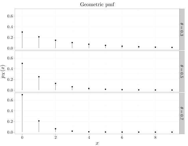
The R code below graphs the pmf of a geometric RV. In accordance with our intuition, it shows that as $\theta$ increases, $X$ is less likely to get high values.
x = 0:9
D = stack(list(`$\\theta=0.3$` = dgeom(x, 0.3), `$\\theta=0.5$` = dgeom(x,
    0.5), `$\\theta=0.7$` = dgeom(x, 0.7)))
names(D) = c("mass", "theta")
D$x = x
qplot(x, mass, data = D, , main = "Geometric pmf",
    geom = "point", stat = "identity", facets = theta ~
        ., xlab = "$x$", ylab = "$p_X(x)$") + geom_linerange(aes(x = x,
    ymin = 0, ymax = mass))