8.6. Law of Large Numbers
Applying Cauchy-Schwartz inequality (Proposition B.4.1) to the inner product $g(X^2,1)=\E(X^2\cdot 1)$ we have that $\E(X^2)^2\leq \E(X^4)$. Similarly, we have $\E(X)^2\leq \E(X^2)$. This shows that $\E(X^r), 1\leq r\leq 4$ is finite if $\E(X^4) < \infty$.
We assume below that $\E(X^{(1)})=0$. We can then prove the general case by applying the obtained result to the sequence $Y^{(n)}=X^{(n)}-\E(X^{(1)})$: $n^{-1}\sum Y^{(n)}\tooas 0$, which implies $n^{-1}\sum X^{(n)}\tooas \E(X^{(1)})$.
We have \begin{align*} \E\left((\sum_{i=1}^n X^{(i)})^4\right) &= \E\left(\sum_{i=1}^n (X^{(i)})^4+6 \sum_{1\leq i < j\leq n} (X^{(i)})^2(X^{(i)})^2\right). \end{align*} The missing terms in the sum above are either $\E(X^{(i)}X^{(j)}X^{(k)}X^{(l)})$ for distinct $i,j,k,l$ or $\E((X^{(i)})^3 X^{(j)})$ for distinct $i,j$. In either case, these terms are zero since expectation of a product of independent RVs is a product of the corresponding expectation, and since $\E(X^{(i)})=0$. The reason for the coefficient 6 is that if we fix the index of the first term in $X^{(a)}X^{(b)}X^{(c)}X^{(d)}$ to be $a=i$, there are three remaining variables that can receive the same index $i$ (the remaining indices get the value $j$). Alternatively, the index of the first variable may be $j$, yielding 3 more terms with the required multiplicity of indices.
This leads to the bound \begin{align*} \E\left(\left(\sum_{i=1}^n X^{(i)}\right)^4\right) &\leq n M + 6 \begin{pmatrix}n\\2\end{pmatrix} M' = nM+3n(n-1)M' \leq n^2 M'' \end{align*} for some finite $M,M',M''<\infty$. Applying Markov's inequality with $k=4$, we get \begin{align*} \P\left(\Big|n^{-1}\sum_{i=1}^n X^{(i)})\Big| \geq \epsilon \right ) = \P\left(\Big|\sum_{i=1}^n X^{(i)})\Big| \geq n \epsilon \right ) \leq M n^{-2}\epsilon^{-4}, \end{align*} which combined with the first Borell-Cantelli lemma (Proposition 6.6.1) shows that \[\P\left(\Big|n^{-1}\sum_{i=1}^n X^{(i)})\Big| \geq \epsilon \text{ i.o.} \right )=0.\] Proposition 8.2.1 completes the proof.
The proposition above remains true under the weaker condition of finite first moment $\E({\bb X}^{(1)}) < \infty$. The proof, however, is considerably more complicated in this case (Billingsley, 1995).
The weak law of large numbers (WLLN) shows that the sequence of random vectors $\bb{Y}^{(n)}=\frac{1}{n}\sum_{i=1}^n\bb{X}^{(i)}$, $n=1,2,\ldots$ is increasingly similar in values to the expectation vector $\bb \mu$. Thus for large $n$, $\bb{Y}^{(n)}$ may be intuitively considered as a deterministic RV whose value is $\mu$ with high probability.
An important special case occurs when $X^{(i)}$ are iid indicator variables $X^{(i)}(\omega)=I_A(\omega)$ with respect to some set $A\subset\R$. In this case, the average $\frac{1}{n}\sum_{i=1}^n\bb{X}^{(i)}=\frac{1}{n}\sum_{i=1}^n I_A$ becomes the relative frequency of occurrence in the set $A$ and the expectation $\E(X^{(i)})$ becomes $\E(I_A)=\P(A)$. We thus have a convergence of relative frequencies as $n\to\infty$ to their expectation.
We demonstrate the WLLN below by drawing samples $X^{(n)}$, $i=1,\ldots,n$ iid from a uniform distribution over $\{1,\ldots,6\}$ (fair die) and displaying $X^{(n)}$ together with the averages $Y^{(n)}=\sum_{i=1}^n X^{(n)}/n$ for different $n$ values.
# draw 10 samples from U({1,...,6})
S = sample(1:6, 10, replace = TRUE)
S
## [1] 2 3 4 6 2 6 6 4 4 1
# compute running averages of 1,...,10 samples
cumsum(S)/1:10
##  [1] 2.000 2.500 3.000 3.750 3.400 3.833 4.143
##  [8] 4.125 4.111 3.800
The example above shows that as $n$ increases, the averages get closer and closer to the expectation 3.5. Below is a graph for larger $n$ values. Note how the variations around 3.5 diminish for large $n$.
S = seq(from = 1, to = 6, length = 200)
par(cex.main = 1.5, cex.axis = 1.2, cex.lab = 1.5)
plot(1:200, S, type = "n", xlab = "$n$", ylab = "$(X_1+\\cdots+X_n)/n$")
for (s in 1:100) lines(1:200, cumsum(sample(1:6, 200,
    replace = TRUE))/1:200, col = rgb(0, 0, 0, alpha = 0.3))
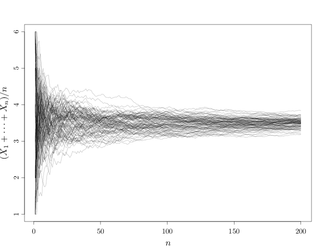
This is one instantiation of the sequence of die rolls. Other instantiations will produce other graphs. The WLLN states that all such graphs will become arbitrarily close to 3.5 as $n$ increases.