$
\def\P{\mathsf{\sf P}}
\def\E{\mathsf{\sf E}}
\def\Var{\mathsf{\sf Var}}
\def\Cov{\mathsf{\sf Cov}}
\def\std{\mathsf{\sf std}}
\def\Cor{\mathsf{\sf Cor}}
\def\R{\mathbb{R}}
\def\c{\,|\,}
\def\bb{\boldsymbol}
\def\diag{\mathsf{\sf diag}}
$
3.14. The Empirical Distribution
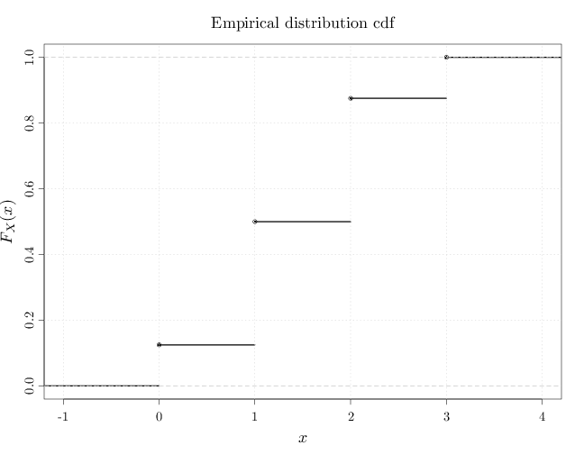
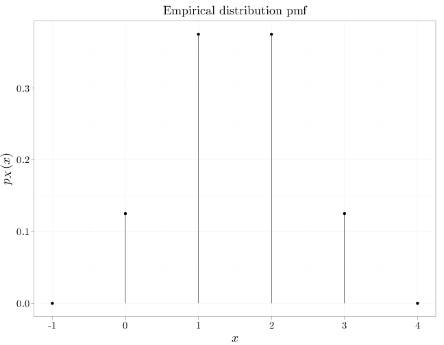
The empirical distribution associated with finite set $A\subset \R$ is a discrete distribution with the following pmf \begin{align*} p_X(x) &= \frac{1}{|A|} \sum_{y\in A} I_{\{y\}} (x), \end{align*} where $I_A(x)=1$ if $x\in A$ and 0 otherwise. In other words, the empirical distribution places equal mass ($1/|A|$) on each of the points in $A$. In some cases, we associate an empirical distribution with a multiset (a set in which some values may appear more than once). Denoting the multiset as a list $A=(y^{(1)},\ldots,y^{(n)})$, $y^{(i)}\in\R$ (we may have $y^{(i)}=y^{(j)}$ for $i\neq j$), the empirical distribution pmf is \begin{align*} p_X(x) &= \frac{1}{n} \sum_{i=1}^n I_{\{y^{(i)}\}} (x). \end{align*} The R code below graphs the pmf and cdf of the empirical distribution associated with $(0,1,1,1,2,2,2,3)$.par(cex.main = 1.5, cex.axis = 1.2, cex.lab = 1.5) D = data.frame(x = c(-1, 0, 1, 2, 3, 4), y = c(0, 1/8, 3/8, 3/8, 1/8, 0)) qplot(x, y, data = D, xlab = "$x$", ylab = "$p_X(x)$", main = "Empirical distribution pmf") + geom_linerange(aes(x = x, ymin = 0, ymax = y))
plot(ecdf(c(0, 1, 1, 1, 2, 2, 2, 3)), verticals = FALSE,
    lwd = 3, xlab = "$x$", ylab = "$F_X(x)$", main = "")
grid()
title(main = "Empirical distribution cdf", font.main = 1)