7.1 Markov Chains
The previous chapter introduced the basic concepts associated with random processes and explored a few basic examples. In this chapter we describe three popular random processes: the Markov chain process, the Poisson process, and the Gaussian process.The previous chapter introduced the basic concepts associated with random processes and explored a few basic examples. In this chapter we explore three popular random processes: the Markov chain process, the Poisson process, and the Gaussian process.
7.1.1 Basic Definitions
Since a Markov chain has Discrete-time, the index set $J$ of the process $\mathcal{X}=\{X_t:t\in J\}$ is finite or countably infinite. We assume that $J=\{0,1,\ldots,l\}$ in the finite case or $J=\{0,1,2,3,\ldots\}$ in the infinite case. Alternative definitions, such as $J=\mathbb{Z}$, lead to similar results but are much less common.
Since a Markov chain has discrete-state, $X_t$ are discrete RVs, or in other words $\P(X_t\in S_t)=1$ for some finite or countably infinite set $S_t$. Taking $S=\cup_t S_t$, we can assume that the random variables $X_t$ have a common discrete state space: $\P(X_t\in S)=1$, for all $t\in J$. Note that $S$ is finite or countably infinite set since it is a countable union of countably infinite sets (see Chapter A). With no loss of generality, we can identify $S$ with $\{0,1,\ldots,l\}$ (in the finite case) or $\{0,1,2,\ldots\}$ (in the countably infinite case). There is no loss of generality since we can simply relabel the elements of the set $S$ with the elements of one of the sets above and adjust the probability function accordingly; for example, $\{\text{red, black, green}\}$ becomes $\{0,1,2\}$.
The Markov assumption implies that for all $k,t$ such that $1\leq k < t \in\mathbb{N}$, we have \begin{align} \tag{*} \P(X_t=x_t \c X_{t-1}=x_{t-1},\ldots,X_{t-k}=x_{t-k})=\P(X_t=x_t \c X_{t-1}=x_{t-1}). \end{align}
Recalling Kolmogorov's extension theorem (Proposition 6.2.1), we can characterize an RP by specifying a consistent set of all finite-dimensional marginal distributions. Together with the Markov assumption (*), this implies that in order to characterize a Markov process $\mathcal{X}$, it is sufficient to specify \begin{align*} T_{ij}(t) &\defeq \P(X_{t+1}=j \c X_{t}=i), & \forall i,j\in S, \forall t\in J \quad & \text{(transition probabilities)}\\ \rho_i &\defeq \P(X_0=i), & \forall i\in S \quad &\text{(initial probabilities)}. \end{align*} The sufficiency follows from the fact that the probabilities above, together with the Markov assumption, are consistent and derive all other finite dimensional marginals. For example, \begin{align*} & \P(X_5=i,X_4=j,X_2=k) \\ &= \P(X_5=i \c X_4=j,X_2=k)\P(X_4=i \c X_2=j)\P(X_2=k) \\ &=\P(X_5=i \c X_4=j)\P(X_4=j \c X_2=k)\P(X_2=k)\\ &=T_{ji}(4) \left(\sum_{l\in S} \P(X_4=j \c X_3=l)\P(X_3=l \c X_2=k)\right)\\ &\qquad\qquad \left(\sum_{r\in S}\sum_{s\in S} \P(X_2=k \c X_1=r)\P(X_1=r \c X_0=s)\P(X_0=s)\right)\\ &=T_{ji}(4)\left(\sum_{l \in S} T_{lj}(3) T_{kl}(2)\right) \left(\sum_{r\in S}\sum_{s\in S} T_{rk}(1) T_{sr}(0) \rho_s\right). \end{align*}
We extend below the definition of the finite dimensional simplex $\mathbb{P}_n$ (Definition 5.2.1) to the countably infinite case below.
We concentrate in the rest of this chapter on Homogenous Markov chains, as they are significantly simpler than the general case.
It is useful to consider the transition probabilities and initial probabilities using algebraic expression. If the state space $S$ is finite, the transition probabilities $T$ form a matrix and the initial probabilities $\bb \rho$ form a vector. If the state space is infinite, the transition probabilities $T$ form a matrix with an infinite number of rows and columns, and the initial probabilities $\bb \rho$ form a vector with an infinite number of components. It is convenient to use matrix algebra to define $TT=T^2$ and ${\bb \rho}^{\top} T$ (the notation ${\bb \rho}^{\top}$ transposes $\bb \rho$ from a column vector to a row vector) as follows: \begin{align*} [ T^2 ]_{ij} &= \sum_{k \in S} T_{ik} T_{kj} \end{align*} \begin{align*} [ {\bb \rho}^{\top} T ]_{i} &= \sum_{k \in S} \rho_k T_{ki}. \end{align*} When the state space $S$ is finite, these algebraic operations reduce to the conventional product between matrices and between a vector and a matrix, as defined in Chapter C. We similarly define higher order powers, such as $T^k=T^{k-1}T$, and also denote $T^0$ as the matrix satisfying $[T^0]_{ij}=1$ if $i=j$ and 0 otherwise (this matrix corresponds to the identity matrix). Note that in the general case $(T_{ij})^n\neq (T^n)_{ij}$. The first term is the $n$-power of a scalar and the second is an element of a matrix raised to the $n$-power. We use the notation $T_{ij}^n$ for the latter: \[ T_{ij}^n \defeq (T^n)_{ij}.\]
Note that the Markov property also implies that \begin{multline*} \P(X_1=x_1,\ldots,X_n=x_n,X_{n+1}=x_{n+1},\ldots,X_{n+m}=x_{n+m} \c X_0=x_0) \\ = \P(X_1=x_2,\ldots,X_n=x_n \c X_0=x_0) \P(X_{1}=x_{n+1},\ldots,X_{m}=x_{n+m} \c X_0=x_n). \end{multline*}
7.1.2 Examples
Assuming $\P(X_0)$ is uniformly distributed over the three states $\rho=(1/3,1/3,1/3)$, The following R code computes the probabilities of $\P(X_t)$ for $t=0,1,\ldots,5$, assuming $\P(X_0)$ is uniformly distributed over the three states: $\rho=(1/3,1/3,1/3)$.
s = factor(c("sunny", "cloudy", "rainy"), levels = c("rainy",
    "cloudy", "sunny"), ordered = TRUE)
P = data.frame(pmf = c(1/3, 1/3, 1/3), state = s, time = "$t=0$")
T = Tk = matrix(c(0.5, 0.4, 0.1, 0.4, 0.5, 0.1, 0.3,
    0.5, 0.2), byrow = T, nrow = 3)
for (i in 2:6) {
    P = rbind(P, data.frame(pmf = t(c(1/3, 1/3, 1/3) %*%
        Tk), state = s, time = rep(paste("$t=", i -
        1, "$", sep = ""), 3)))
    Tk = Tk %*% T
}
P
##       pmf  state  time
## 1  0.3333  sunny $t=0$
## 2  0.3333 cloudy $t=0$
## 3  0.3333  rainy $t=0$
## 4  0.4000  sunny $t=1$
## 5  0.4667 cloudy $t=1$
## 6  0.1333  rainy $t=1$
## 7  0.4267  sunny $t=2$
## 8  0.4600 cloudy $t=2$
## 9  0.1133  rainy $t=2$
## 10 0.4313  sunny $t=3$
## 11 0.4573 cloudy $t=3$
## 12 0.1113  rainy $t=3$
## 13 0.4320  sunny $t=4$
## 14 0.4569 cloudy $t=4$
## 15 0.1111  rainy $t=4$
## 16 0.4321  sunny $t=5$
## 17 0.4568 cloudy $t=5$
## 18 0.1111  rainy $t=5$
The numeric results above are displayed in a graph below.
qplot(x = state, ymin = 0, ymax = pmf, data = P, geom = "linerange",
    facets = "time~.", ylab = "$p_{X_t}$") + geom_point(aes(x = state,
    y = pmf)) + coord_flip()
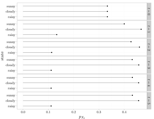
We observe that (i) even though the initial weather $X_0$ is uniformly distributed over the three states, the weather at time $t=5$ is highly unlikely to be rainy, and (ii) it appears that \[ \lim_{t\to\infty} p_{X_t}(r) = \begin{cases} 0.4321 & r=\text{sunny}\\ 0.4558 & r=\text{cloudy} \\ 0.1111 & r=\text{rainy}\end{cases}. \] We will confirm this experimental observation with theory later in this section when we discuss the stationary distribution.
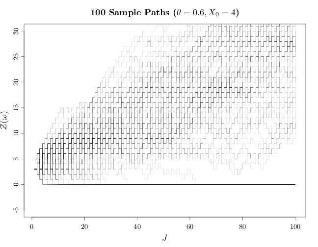
This Markov chain corresponds to the random walk model described in Section 6.4. The random variable $X_t$ denotes the capital of a persistent gambler that wins 1 dollar with probability $\theta$ and loses 1 dollar with probability $1-\theta$. It is assumed that the gambler starts with zero capital and is able to keep accumulating debt indefinitely if needed.
The state space in this case is $S=\{0,1,2,\ldots\}$, the initial probabilities are $\rho_k=1$ and $\rho_j=0$ for $j\neq k$, and the transition probabilities are \[ T_{ij} = \begin{cases} 1 & i = 0 = j\\ 0 & i = 0 < j\\ \theta & j=i+1 > 1\\ 1-\theta & j = i - 1 > 0\\ 0 & \text{otherwise} \end{cases}. \]
The R code graphs 100 sample paths for $\theta=0.6$. We use transparency in order to illustrate regions where many sample paths overlap. Such regions are shaded darker than regions with a single sample path or a few overlapping paths.
J = 1:100
par(cex.main = 1.5, cex.axis = 1.2, cex.lab = 1.5)
plot(c(1, 100), c(-5, 30), type = "n", xlab = "$J$",
    ylab = "$\\mathcal{Z}(\\omega)$")
Zn100 <- Zn500 <- vector(len = 100)
for (i in 1:100) {
    X = rbinom(n = 500, size = 1, prob = 0.6)
    Z = cumsum(2 * X - 1) + 4
    Z[cumsum(Z == 0) > 0] = 0
    lines(J, c(Z[1:100]), type = "s", col = rgb(0,
        0, 0, alpha = 0.2))
    Zn100[i] = Z[100]
    Zn500[i] = Z[500]
}
title("100 Sample Paths ($\\theta=0.6, X_0=4$)")
The R code below graphs a histogram of the capital of the random gambler at $t=100$ over multiple samples. The shape of the histogram approximates $p_{X_t}$.
qplot(Zn100, main = "histogram (100 sample paths)",
    xlab = "$Z_{100}$")
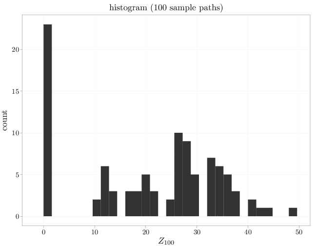
Comparing the graph above with the graph in Section 6.4 we see that the gambler (usually) does much worse in the graphs above than in the case of Section 6.4, even though the gambler starts with 4 dollars instead of 0 dollars.
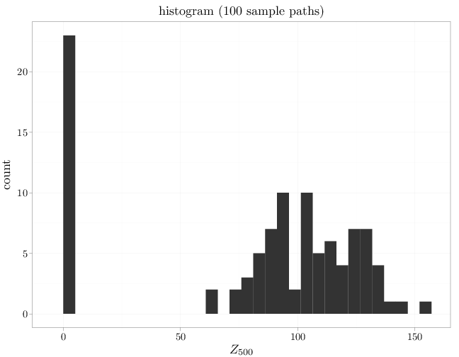
Repeating the previous graph for $t=500$ below, we see that the two groups (ruined gamblers and newly rich gamblers) become more separated.
qplot(Zn500, main = "histogram (100 sample paths)",
    xlab = "$Z_{500}$")
7.1.3 Transience, Persistence, and Irreducibility
Note that the sequence of probabilities $f_{ij}^{(n)}$, $n\in\mathbb{N}$ correspond to a sequence of disjoint events, implying that the sum $f_{ij}$ corresponds to the probability of their union.
The notation i.o. above corresponds to infinitely often (see Section A.4).
It remains to show that $f_{ss} < 1$ implies $\sum_n T_{ss}^n < \infty$. Consider the event of transitioning from state $s$ to state $s'$ after $n$ steps. The first time the chain visits $s'$ may occur after 1 time step, after 2 time steps, and so on until $n$ time steps. Using the law of total probability (Proposition 1.5.4) we have \begin{align*} T_{ss'}^{n} &= \sum_{r=0}^{n-1} f_{ss'}^{(n-r)} T_{s's'}^{r}\\ \sum_{t=1}^n T_{ss}^{t} &= \sum_{t=1}^n \sum_{r=0}^{t-1} f_{ss'}^{(n-r)} T_{s's'}^{r} \\ &= \sum_{r=0}^{n-1} \sum_{t=r+1}^n f_{ss'}^{(n-r)} T_{s's'}^{r} \\ &= \sum_{r=0}^{n-1} T_{s's'}^{r} \sum_{t=r+1}^n f_{ss'}^{(n-r)} \\ &\leq f_{ss} \sum_{r=0}^n T_{ss}^{r}\\ (1-f_{ss}) \sum_{t=1}^n T_{ss}^{t} &\leq f_{ss}. \end{align*} The third equality follows from the fact that the double summation ranges over the indices \[\{t,r: 1 \leq t\leq n, 0\leq r < t\}=\{t,r: r< t\leq n, 0\leq r\leq n-1\}.\] The last inequality above follows from the fact that $T_{ss}^{0}=1$. This shows that $f_{ss}<1$ implies $\sum_n T_{ss}^n<\infty$ and concludes the proof of (i).
The proof of (ii) follows from the proof of (i) and the fact that $\P(X_n=s\text{ i.o.} \c X_0=s)=0$ is either 0 or 1, $\sum_{n\in\mathbb{N}} T_{ii}^n$ is either finite or infinite, and a state is either persistent or transient.
- (i) All states are transient, $\P(\cup_{s\in S} \{X_n=s \text{ i.o }\} \c X_0=s')=0$ for all $s'\in S$, and $\sum_{n\in\mathbb{N}} T_{ss'}^n<\infty$.
- (ii) All states are persistent, $\P(\cap_{s\in S} \{X_n=s \text{ i.o }\} \c X_0=s')=1$ for all $s'\in S$, and $\sum_{n\in\mathbb{N}} T_{ss'}^n=+\infty$.
If all states are transient, then by Proposition 7.1.3 $\P(X_n=s \text{ i.o } \c X_0=s')=0$ for all $s,s'\in S$ and $\P(\cup_{s\in S} \{X_n=s \text{ i.o }\} \c X_0=s')=0$ (as implied by Proposition 1.6.8, a countable union of sets with zero probability have zero probability). Denoting the time of first transition from $s$ to $s'$ by $r$, the law of total probability (Proposition 1.5.4) implies \begin{align*} \sum_{n=1}^{\infty} T_{ss'}^n &= \sum_{n=1}^{\infty} \sum_{r=1}^n f_{ss'}^{(r)} T_{s's'}^{n-r} \\ &= \sum_{r=1}^{\infty}f_{ss'}^{(r)} \sum_{m=1}^{\infty}T_{s's'}^{m} \\ &\leq \sum_{m=1}^{\infty}T_{s's'}^{m}. \end{align*} Since the states are transient, Proposition 7.1.4 implies that $\sum_{m=1}^{\infty}T_{s's'}^{m} < \infty$, which together with the inequality above implies $\sum_{n=1}^{\infty} T_{ss'}^n < \infty$.
If all states are persistent, Proposition 7.1.4 implies that $\P(X_n=s \text{ i.o } \c X_0=s')=0$ and \begin{align*} T_{ss'}^m &= \P(X_m=s' \c X_0=s)\\ &= \P(\{X_m=s'\}\cap \{X_n=s\text{ i.o }\} \c X_0=s) \\ &\leq \sum_{n=m+1}^{\infty} \P( X_m=s', X_{m+1}\neq s,\ldots, X_{n-1}\neq s,X_m=s \c X_0=s)\\ &=\sum_{n=m+1}^{\infty} T_{ss'}^m f_{s's}^{(n-m)}\\ &= f_{s's} \sum_{n=m+1}^{\infty} T_{ss'}^m. \end{align*}
By irreducibility, there exists $m$ for which $T_{ss'}^m>0$, implying that $f_{ss'}>0$, which can only happen if $f_{ss'}=1$. Since we did not constrain the choice of $s,s'$, we have $f_{ss'}=1$ for all $s,s'\in S$. This implies $\P(X_n=s \text{ i.o } \c X_0=s')=1$ for all $s,s'$, and by de-Morgan's law \begin{align*} \P(\cap_{s\in S} \{X_n=s \text{ i.o }\} \c X_0=s')&= 1-\P(\cup_{s\in S} \{X_n=s \text{ i.o }\}^c \c X_0=s')\\ &\geq 1-\sum_{s\in S} \P(\{X_n=s \text{ i.o }\}^c \c X_0=s')) \\ &= 1-0. \end{align*} Finally, $\sum_{n\in\mathbb{N}} T_{ss'}^n=+\infty$ since otherwise Proposition 6.6.1 would imply that $\P(X_n=s \text{ i.o } \c X_0=s')=0$, yielding a contradiction.
Since for an irreducible Markov chain, all states are persistent or transient we refer to the Markov chain itself as persistent or transient.
7.1.4 Persistence and Transience of the Random Walk Process
The Markov chain corresponding to the symmetric random walk on $\mathbb{Z}^d$ (Example 7.1.5) is persistent when $d=1$ or $d=2$ and transient for $d\geq 3$. This is a remarkable result since it shows a qualitatively different behavior between the cases of one and two dimensions on one hand and three or more dimensions on the other hand.By a symmetry argument, the probability $T_{ss}^n$ is the same for all $s\in S$ and so we denote it as $q_{n}^{(d)}$.
If $d=1$, a return to the starting point after $n$ step is possible only if $n$ is even. We compute below $q_{2n}^{(d)}$, $n\in\mathbb{N}$ ($q_{2n+1}^{(d)}=0$ since $2n+1$ is odd). We have \[q_{2n}^{(d)}=\begin{pmatrix}2n\\n\end{pmatrix} 2^{-2n}\] since there are $2n$-choose $n$ ways to select $n$ moves to the right and the remaining moves are automatically chosen as moves to the left, and each such sequence of moves occurs with probability $(1/2)^{2n}$. Using Stirling's Formula (Proposition 1.6.2), we have \begin{align*} q_{n}^{(1)} &= \frac{(2n)!}{n!n!} 2^{-2n} \\ &= \frac{(2n)!}{(2n)^{2n+1/2} e^{-2n}} \cdot \frac{n^{n+1/2} e^{-n}}{n!} \cdot \frac{(2n)^{2n+1/2} e^{-2n}}{n^{2n+1} e^{-2n}} 2^{-2n}\\ &= \frac{(2n)!}{(2n)^{2n+1/2} e^{-2n}} \cdot \frac{n^{n+1/2} e^{-n}}{n!} \cdot 2^{1/2} n^{-1/2} \\ &\sim (\pi n)^{-1/2}. \end{align*} (See Section B.5 for an explanation of the notation $\sim$ above.) It follows from Proposition D.2.5 that $\sum_{n\in\mathbb{N}} q_{n}^{(1)}=\infty$, implying that the chain is persistent.
If $d=2$, a return to the starting point after $2n+1$, $n\in\mathbb{N}$ steps is impossible. A return to the starting point after $2n, n\in\mathbb{N}$ is possible only if the number of up and down steps are equal and the number of right and left steps are equal. The number of such sequences of length $2n$ multiplied by their probability $(1/4)^{-2n}$ gives \begin{align} q_{2n}^{(2)} &= \sum_{r=0}^n \frac{(2n)!}{r!r!(n-r)!(n-r)!} \frac{1}{4^{2n}} \\ &= 4^{-2n} \begin{pmatrix} 2n\\n\end{pmatrix} \sum_{r=0}^n \begin{pmatrix} n\\u\end{pmatrix} \begin{pmatrix} n\\n-u\end{pmatrix}\\ &=4^{-2n} \begin{pmatrix} 2n\\n\end{pmatrix}\begin{pmatrix} 2n\\n\end{pmatrix}. \tag{**} \end{align} The first equality above follows from Proposition 1.6.7, where $r$ corresponds to the number of up moves and $n-r$ corresponds to the number of right moves. The last equality above holds since $\sum_{r=0}^n \begin{pmatrix} n\\u\end{pmatrix} \begin{pmatrix} n\\n-u\end{pmatrix}$ is the number of possible ways to select $n$ out of $2n$ with no replacement and no order: first select $u$ from the first half containing $n$ items and then select $n-u$ items from the second half containing $n$ items, for all possible values of $u$: $0\leq u\leq n$. As in the case of $d=1$, using Stirling's approximation on (**) yields $q_{2n}^{(d)}\sim (\pi n)^{-1}$. As before, Proposition D.2.5 leads then to $\sum_{n\in\mathbb{N}} q_{n}^{(2)}=\infty$ implying that the chain is persistent.
If $d=3$ similar arguments lead to \begin{align*} q_{2n}^{(3)} &= \sum \frac{(2n)!}{r!r!q!q!(n-r-q)!(n-r-q)!} \frac{1}{6^{2n}} \end{align*} where the sum ranges over all non-negative $r,q$ satisfying $r+q\leq n$ ($r$ is the number of steps up, $q$ the number of steps right, and $n-r-q$ the number of steps in the third dimension). Conditioning on the number of moves in the third dimension, we can reduce the above equation to quantities containing $q_n^{(1)}$ and $q_n^{(2)}$: \begin{align} q_{2n}^{(3)} &= \sum_{l=0}^n \begin{pmatrix} 2n\\ 2l\end{pmatrix} \left(\frac{1}{3}\right)^{2n-2l} \left(\frac{2}{3}\right)^{2l} q_{2n-2l}^{(1)}\,q_{2l}^{(2)}. \end{align} By bounding the above terms, it can be shown that $q_{2n}^{(3)}=O(n^{-3/2})$ (details are available at (Billingsley, 1995, Example 8.6) which implies (see Proposition D.2.5) $\sum_{n\in\mathbb{N}} q_{n}^{(2)} < \infty$, showing that the Markov chain is transient. Similar recursive arguments for $d > 3$ lead to $q_{n}^d=O(n^{-k/2})$, implying (see Proposition D.2.5) $\sum_{n\in\mathbb{N}} q_{n}^{(d)} < \infty$, for $d\geq 3$, and consequentially showing the transience for dimensions higher than 3.
7.1.5 Periodicity in Markov Chains
As a result of the above proposition, we refer to the common period as the period of the Markov chain. If it is 1, we say that the Markov chain is aperiodic.
We define $A'=\{a-b:a,b\in A\}\cup A\cup \{-a:a\in A\}$ and refer to the smallest positive element of $A'$ as $d$. For $x\in A'$, we have $x=qd+r$, $0\leq q < d$. Since $A'$ is closed under addition and subtraction $r=x-qd\in A'$ and since $d$ is the smallest positive element in $A'$, we have $r=0$. This implies that $A'$ contains all multiples of $d$. Consequentially, $d$ divides all elements in $A'$ and therefore all element in $A$, implying that $d=1$ (since $A$ is a set with a greatest common divisor of 1). We thus have $1\in A'$ expressed as $1=x-y$ for $x,y\in A$. We show next that $A$ contains all elements greater than $N'=(x+y)^2$. For $a> N'$ we write $a=q(x+y)+r$ for some $q$ and $0\leq r < x+y$. Since $a > N'\geq(r+1)(x+y)$, we have $q=(a-r)/(x+y) > r$ implying that $q+r\geq q-r > 0$. This leads to \[a=q(x+y)+r= q(x+y)+r(x-y)=(q+r)x+(q-r)y, \qquad q+r>0, \quad q-r>0,\] which together with the fact that $A$ is closed under addition implies that $a\in A$. This concludes the proof that $A$ contains all integers greater than $N'$.
We denote the set of $n\in\mathbb{N}$ for which $T_{s's'}^n>0$ by $A$. Since $T_{s's'}^{a+b}\geq T_{s's'}^aT_{s's'}^b$, it follows that $A$ is closed under addition. Since the chain is aperiodic, it follows that $A$ has a greatest common divisor of 1. Using the result above, we have that $A$ contains all integers greater than $N'$. Setting $N=N'+r$, where $T_{ss'}^r>0$ we have than whenever $n>N$, $T_{ss'}^n\geq T_{ss'}^rT_{s's'}^{n-r}> 0$.
7.1.6 The Stationary Distribution
Using algebraic notation, we may treat $T$ as a (potentially infinite) matrix and $\bb q=(q(s):s\in S)$ as a (potentially infinite) column vector. The first condition above then becomes \begin{align*} {\bb q}^{\top}T ={\bb q}^{\top} \qquad \text{or} \qquad T^{\top}\bb q=\bb q \end{align*} implying that $\bb q$ is an eigenvector of the matrix $T^{\top}$ with eigenvalue 1. The second and third conditions in the definition above ensures that $\bb q$ represents a distribution over $S$. Note that if $\bb q$ corresponds to the stationary distribution of a Markov chain, then we have \[ (T^k)^{\top}\bb q=\bb q, \qquad \forall q\in\mathbb{N}.\]
We construct a new Markov chain process with a state space $S\times S$ and transition probabilities $\tilde{T}_{sr,s'r'}=T_{ss'}T_{rr'}$. Note that $\tilde T$ indeed represents transition probabilities since it is non-negative and \[\sum_{s'}\sum_{r'} \tilde{T}_{sr,s'r'}=\sum_{s'}T_{ss'}\sum_{r'}T_{rr'}=1.\] The new Markov chain represents two independent Markov chains processes progressing in parallel, and so ${\tilde T}^n_{sr,s'r'}=T_{ss'}^nT_{rr'}^n$.
Since the two independent Markov chains are irreducible, there exists $N$ such that $n > N$ implies $T_{ss'}^nT_{rr'}^n$ is positive (Proposition 7.1.6), implying that ${\tilde T}^n_{sr,s'r'}$ for $n>N$, making the new coupled Markov chain irreducible. The aperiodicity of the original Markov chain implies that the coupled Markov chain is aperiodic as well. The function $q(s,r)=q(s)q(r)$ on $S\times S$ is a stationary distribution of the new Markov chain: \begin{align*} \sum_{s,r} q(s,r) \tilde{T}_{sr,s'r'} &= \sum_{s,r} q(s) q(r) T_{ss'} T_{rr'} \\ &= \sum_{s} q(s) T_{ss'} \sum_{r} q(r) T_{rr'} \\ &= q(s')q(r') \\ &= q(s',r')\\ \sum_{s,r} q(s,r) &= \sum_r q(s)\sum_s q(s)=1\cdot 1\\ q(s,r)&=q(s)q(r)\geq 0. \end{align*} Since the coupled Markov chain is aperiodic, irreducible and has a stationary distribution, it is also persistent.
Denoting the two component Markov chains composing the coupled chain by $X_n$ and $Y_n$, and $\tau=\min \{n: X_n=Y_n=c\}$ (note that since the coupled chain is persistent, it visits $(c,c)$ i.o. and therefore $\tau$ is finite), we have \begin{multline*} \P(X_n=r,Y_n=r',\tau=m \c X_0=s,Y_0=s') \\ = \P(\tau=m \c X_0=s,Y_0=s') T_{cr}^{n-m} T_{cr'}^{n-m}, \qquad m\leq n. \end{multline*} Summing over all possible values of $r'$ in the equation above gives $\P(X_n=r,\tau=m \c X_0=s,Y_0=s') = \P(\tau=m \c X_0=s,Y_0=s') T_{cr}^{n-m}$ and summing over all possible values of $r$ in the equation above gives $\P(Y_n=r',\tau=m \c X_0=s,Y_0=s') = \P(\tau=m \c X_0=s,Y_0=s') T_{cr'}^{n-m}$. Setting $r=r'$ and summing over $m=1,2,\ldots,n$ we get \begin{align*} \P(Y_n=r,\tau\leq m \c X_0=s,Y_0=s') = \P(X_n=r,\tau\leq m \c X_0=s,Y_0=s'). \end{align*} Thus, even though the two chains started from different states $s$ and $s'$, conditioned on the chains meeting at $\tau$, their distributions for times $n\geq \tau$ are identical.
We have \begin{align*} &\P(X_n=r \c X_0=s,Y_0=s') \\ &= \P(X_n=r, \tau \leq n \c X_0=s,Y_0=s') + \P(X_n=r, \tau > n \c X_0=s,Y_0=s')\\ &\leq \P(X_n=r, \tau \leq n \c X_0=s,Y_0=s') + \P(\tau > n \c X_0=s,Y_0=s')\\ &= \P(Y_n=r, \tau \leq n \c X_0=s,Y_0=s') + \P(\tau > n \c X_0=s,Y_0=s')\\ &\leq \P(Y_n=r \c X_0=s,Y_0=s') + \P(\tau > n \c X_0=s,Y_0=s'). \end{align*} Repeating the equation above with $X_n$ and $Y_n$ interchanged yields \begin{align} \notag |T_{sr}^n-T_{s'r}^n| &= |\P(X_n=r \c X_0=s,Y_0=s') -\P(Y_n=r \c X_0=s,Y_0=s') |\\ &\leq \P(\tau > n \c X_0=s,Y_0=s').\tag{***} \end{align} Since $\tau$ is finite, the right hand side above converges to 0 (as $n\to\infty$), implying that the left hand side also converges to 0. \begin{align*} \lim_{n\to\infty} |T_{sr}^n-T_{s'r}^n|=|\P(X_n=r \c X_0=s,Y_0=s') -\P(Y_n=r \c X_0=s,Y_0=s') | =0. \end{align*} Again, this implies that the two chains "mix" or behave identically for large $n$ even though they started from different initial states.
Using the fact that $q$ is the stationary distribution of the chain we have \[ \rho(r) -T_{s'r}^n = \sum_{s\in S} \rho(s)T_{sr}^n - 1\cdot T_{s'r}^n = \sum_{s\in S} \rho(s)(T_{sr}^n-T_{s'r}^n),\] which converges to 0 by (***). To show that $q$ is positive, we let $r\to\infty$ in the following inequality \[ T_{ss}^{(n+m+r)} \geq T_{ss'}^n T_{s's'}^r T_{s's}^m,\] yielding \[ q(s) \geq T_{ss'}^n q(s') T_{s's}^m.\] Since the chain is persistent we can choose $n$ and $m$ such that $T_{ss'}^n>0$ and $T_{s's}^m>0$. It thus follows that if $q(s')$ is positive then $q(s)$ is positive. Since $\sum q(s)=1$, we have that $q(s)>0$ for all $s\in S$.
The stationary distribution is extremely important in understanding the behavior of Markov chains (it if exists). As the following corollary shows, the distribution of $X_n$ for large $n$ will converge to the stationary distribution. In particular, this occurs regardless of the initial probabilities $\P(X_0)$. In other words, for large $n$, the distribution of $X_n$ is approximately independent of $n$ and is approximately independent of the initial distribution $\rho$ or the initial state $X_0$. Algebraically, this implies that the rows of $T^n$ converge to the vector $\bb q$ and thus \[\lim_{n\to\infty} {\bb\rho}^{\top} T^n = \bb q, \qquad \forall \bb \rho\in \mathbb{P}_S.\]
library(expm)
print(T <- matrix(c(0.5, 0.4, 0.1, 0.4, 0.5, 0.1, 0.3,
    0.5, 0.2), byrow = T, nrow = 3))
##      [,1] [,2] [,3]
## [1,]  0.5  0.4  0.1
## [2,]  0.4  0.5  0.1
## [3,]  0.3  0.5  0.2
print(q <- c(0.4321, 0.4558, 0.1111))
## [1] 0.4321 0.4558 0.1111
# verify that q is a stationary distribution
sum(q)
## [1] 0.999
c(0.4321, 0.4558, 0.1111) %*% T
##        [,1]   [,2]  [,3]
## [1,] 0.4317 0.4563 0.111
# raise transition matrix to the 10 power
print(T10 <- T %^% 10)
##        [,1]   [,2]   [,3]
## [1,] 0.4321 0.4568 0.1111
## [2,] 0.4321 0.4568 0.1111
## [3,] 0.4321 0.4568 0.1111
# distribution of chain at t=10 for 3 different
# initial distributions
c(1, 0, 0) %*% T10
##        [,1]   [,2]   [,3]
## [1,] 0.4321 0.4568 0.1111
c(0, 1, 0) %*% T10
##        [,1]   [,2]   [,3]
## [1,] 0.4321 0.4568 0.1111
c(0, 0, 1) %*% T10
##        [,1]   [,2]   [,3]
## [1,] 0.4321 0.4568 0.1111