Probability
The Analysis of Data, volume 1
Relationship between Integration and Differentiation
$
\def\P{\mathsf{\sf P}}
\def\E{\mathsf{\sf E}}
\def\Var{\mathsf{\sf Var}}
\def\Cov{\mathsf{\sf Cov}}
\def\std{\mathsf{\sf std}}
\def\Cor{\mathsf{\sf Cor}}
\def\R{\mathbb{R}}
\def\c{\,|\,}
\def\bb{\boldsymbol}
\def\diag{\mathsf{\sf diag}}
\def\defeq{\stackrel{\tiny\text{def}}{=}}
$
F.2. Relationship between Integration and Differentiation
As the following results indicate, integration and differentiation are in some sense opposite operations.
Proposition F.2.1.
Let $f:[a,b]\to\R$ be a bounded function and $P$ a partition of $[a,b]$ such that
$U(P,f)-L(P,f) < \epsilon$. Then
\[ \Bigg| \sum_{i=1}^n f(t_i)|\Delta_i| - \int_a^b f\,dx \Bigg| < \epsilon, \qquad \forall t_i\in\Delta_i,\,\, i=1,\ldots,n.\]
Proof.
The proposition follows from the fact that both $\sum_{i=1}^n f(t_i) |\Delta_i|$ and $\int_a^b f\,dx$ lie in the interval
$[L(P,f), U(P,f)]$, whose length is $\epsilon$.
The following proposition formulates a very important connection between differentiation and integration. It leads to many useful integration techniques, and is important in probability theory in formulating a connection between the cdf and pdf of a continuous random variable.
Proposition F.2.2 (The Fundamental Theorem of Calculus). Part 1: Let $f:[a,b]\to\R$ be a bounded integrable function. Then
(i) $F(x)=\int_a^x f(t)\,dt$ is a continuous function on $[a,b]$, and (ii) if $f$ is continuous then $F$ is differentiable and
\[F'(x) = \frac{d}{dx}\int_a^x f(t)\,dt=f(x).\]
Part 2: For any differentiable function $F$ whose derivative $F'(t)=f(t)$ is Riemann integrable,
\begin{align*}
F(b)-F(a) = \int_{a}^b f(t)\, dt.
\end{align*}
In the second part of the proposition above, the function $F$ is called the anti-derivative of $f$. The second part of the proposition thus provides an easy way to compute the integral $\int_{a}^b f(t)\, dt$ of a function $f$ with a known anti-derivative $F$.
Proof.
We first prove part 1. For $x < y$ we have
\[ |F(y)-F(x)|=\Big| \int_x^y f(t)\,dt \Big| \leq (y-x) \sup_{t\in [a,b]} |f(t)|.\]
Thus for all $\epsilon>0$, if $|y-x| < \delta=\epsilon/ \sup_{t\in [a,b]} |f(t)|$ then $|F(y)-F(x)| < \epsilon$ showing (i).
If $f$ is continuous on $[a,b]$ then it is also uniformly continuous, and for all $\epsilon>0$ we can select $\delta>0$ such that $|x-x_0| < \delta$ implies $|f(x)-f(x_0)| < \epsilon$. It follows that
\[ \Big|\frac{F(x)-F(x_0)}{x-x_0}-f(x_0)\Big| = \Big| (x-x_0)^{-1} \int_{x_0}^x (f(r)-f(x_0) )\,dr \Big| \leq \epsilon,\]
which implies (ii).
We now prove part 2. Given $\epsilon>0$ we construct a partition $P=\{x_0,\ldots,x_n\}$ such that $U(P,f)-L(P,f) < \epsilon$. By the mean value theorem (Proposition D.1.5) there exists a point $r_i\in(x_{i-1},x_i)$ such that \[F(x_i)-F(x_{i-1})=f(r_i)\Delta_i, \quad i=1,\ldots,n.\] Summing the above equations for all $i$ we get
\[ F(b)-F(a) = \sum_{i=1}^n f(r_i) |\Delta_i|\]
and using Proposition F.2.1 we have
\[ \Big| F(b)-F(a) -\int_a^b f(x)\,dx \Big| < \epsilon.\]
Since $\epsilon>0$ is arbitrary, the proposition follows.
Example F.2.1.
Since $cx^{n+1}/(n+1)$ is the anti-derivative of $cx^n$,
\begin{align*}
\int_a^b cx^{n} \,dx = \frac{c}{n+1}x^{n+1}\Big|_a^b=\frac{c}{n+1}(b^{n+1}-a^{n+1}).
\end{align*}
Example F.2.2.
Since $(1/c)e^{cx}$ is the anti-derivative of $e^{cx}$,
\begin{align*}
\int_a^b e^{cx} \, dx = (1/c)e^{cx}\Big|_a^b=(1/c)\left(e^{cb}-e^{ca}\right).
\end{align*}
For example
\begin{align*}
\int_0^{\infty} e^{-r/2} \, dr = \left(-2 e^{-r/2}\right) \Big|_0^{\infty} = -2 (0-1)=2.
\end{align*}
Proposition F.2.3 (Change of Variables). Let $g$ be a strictly monotonic increasing and differentiable function whose derivative $g'$ is continuous on $[a,b]$ and $f$ be a continuous function. Then
\[\int_{g(a)}^{g(b)} f(t)\,dt = \int_{a}^{b} f(g(t)) g'(t) \,dt.\]
Proof.
Since $f,g,g'$ are continuous, $f(g(t))g'(t)$ is continuous as well and therefore Riemann integrable. Defining $F(t)=\int_{g(a)}^t f(t)\,dt$, we have
\begin{align*}
\int_a^b f(g(t))g'(t)\,dt &= \int_a^b F'(g(t))g'(t)\, dt\\
&=\int_a^b (F\circ g)'(t)\,dt \\
&= (F\circ g)(b)-(F\circ g)(a) \\
&=\int_{g(a)}^{g(b)} f(t)\,dt.
\end{align*}
Above, we used the first part of the fundamental theorem of calculus in first equality, the differentiation chain rule in the second equality, and the second part of the fundamental theorem of calculus in the third and fourth equalities.
In many cases the integral on the right hand side above is difficult to compute but the integral on the left hand side is easier. In these cases the change of variables provides a useful tool for computing integrals.
Example F.2.3.
Using the variable transformation $y=f(x)=(x-\mu)/\sigma$, $f'(x)=1/\sigma$, and
\begin{align*}
\int_{(a-\mu)/\sigma}^{(b-\mu)/\sigma} \exp\left(-\frac{y^2}{2}\right) \,dy = \int_{a}^{b}\exp\left(-\frac{(x-\mu)^2}{2\sigma^2} \right) \,\frac{1}{\sigma}dx.
\end{align*}
We compute the integral on the left hand side in Example F.6.1 (for $a\to-\infty, b\to\infty$).
Example F.2.4.
Using the variable transformation $y=f(x)=-x^2/2$ with $f'(x)=-x$,
\begin{align}
\int_a^{b} e^{-x^2/2}\,(-x) dx = \int_{-a^2/2}^{-b^2/2} e^{y} \, dy = e^{-b^2/2}-e^{-a^2/2}.
\end{align}
where the left hand side above corresponds to the right hand side in Proposition F.2.3. For example,
\begin{align}
\int_0^{\infty} e^{-x^2/2}\, x dx = - \int_{0}^{-\infty} e^{y} \, dy = -(e^y)\Big|_0^{-\infty}=-(0-1)=1.
\end{align}
Proposition F.2.4 (Integration by Parts)/
For two differentiable functions $f,g:\R\to\R$ we have
\[ \int_a^b f(x)g'(x)\, dx = f(b)g(b)-f(a)g(a)-\int_a^b f'(x)g(x)\, dx.\]
Proof.
The result follows from the second part of the Fundamental Theorem of Calculus (Proposition F.2.2), applied to $h(x)=f(x)g(x)$ and its derivative $h'=f'g+g'f$.
Example F.2.5.
\begin{align*}
\int_a^{b} x^{c}e^{-x}\, dx &=
\left(-x^c e^{-x}\right)\Big|_a^{b}
- c \int_a^{b} x^{c-1} e^{-x}\, dx.
\end{align*}
For example, the integral below known as the Gamma function satisfies for $c>1$
\begin{align*}
\Gamma(c) &\defeq \int_0^{\infty} x^{c-1}e^{-x}\, dx \\ &=
\left(-x^{c-1} e^{-x}\right)\Big|_0^{\infty}
- \left(-(c-1) \int_0^{\infty} x^{c-2} e^{-x}\, dx\right) \\ &=
(0-0) + (c-1) \int_0^{\infty} x^{c-2} e^{-x}\, dx \\ &=(c-1)\Gamma(c-1).
\end{align*}
where the last equality follows from L'Hospital's rule (Proposition D.1.7) that implies $\lim_{x\to\infty} x^{c-1}/e^{x}=0$ for $c>1$ (the limit $\lim_{x\to 0} x^{c-1}/e^{x}=0$ follows from the facts that $x^{c-1}\to 0$ and $e^x\to 1$ and division is a continuous function that preserves limits). Applying the above equation recursively together with
\[ \Gamma(1)=\int_0^{\infty} \exp(-t)\, dt = \left(-e^{-t}\right)\Big|_0^{\infty}=1-0=1,\]
we get
\[\Gamma(n)=(n-1)!, \qquad n\in\mathbb{N}.\]
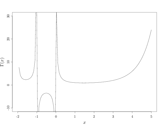
Thus, for $x > 1$ the Gamma function extends the factorial function from the natural numbers to real values $x > 1$. The R code below graphs the Gamma function for the positive reals, as well as for negative values. The graph exhibits an unexpected behavior for $x<1$, specifically: a non-monotonic behavior for $x < 1$ and discontinuities at non-positive integers.
par(cex.main = 1.5, cex.axis = 1.2, cex.lab = 1.5)
plot.function(gamma, from = -2, to = 5, xlab = "$x$",
    ylab = "$\\Gamma(x)$", ylim = c(-10, 30))