$
\def\P{\mathsf{\sf P}}
\def\E{\mathsf{\sf E}}
\def\Var{\mathsf{\sf Var}}
\def\Cov{\mathsf{\sf Cov}}
\def\std{\mathsf{\sf std}}
\def\Cor{\mathsf{\sf Cor}}
\def\R{\mathbb{R}}
\def\c{\,|\,}
\def\bb{\boldsymbol}
\def\diag{\mathsf{\sf diag}}
$
3.7. The Uniform Distribution
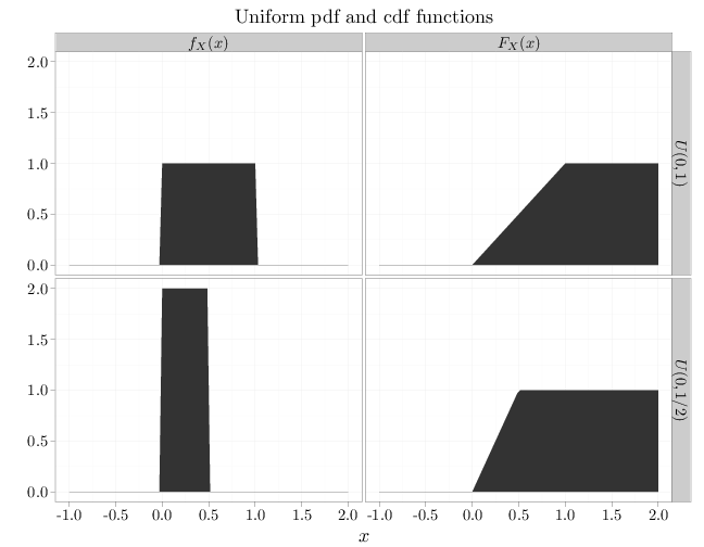
The uniform RV, $X\sim U(a,b)$, where $a < b$, is the classical model on the interval $[a,b]$ (see Section 1.4). By definition, the pdf of a $U(a,b)$ RV is constant for $x\in[a,b]$ and 0 for $x\not\in[a,b]$. The only such constant function that integrates to one is $f(x)=1/(b-a)$ for $x\in [a,b]$ and 0 otherwise, implying that \[f_X(x)=\begin{cases}1/(b-a) & x\in[a,b]\\ 0 & \text{otherwise}\end{cases}.\]
As computed in Example 2.3.2, \begin{align*} \E(X)&=(a+b)/2\\ \Var(X)&=(b-a)^2/12 \end{align*} implying that the expectation is the mid-point of the interval and the variance increases with the square of the interval width. The R code below graphs the pdf and the cdf of $U(a,b)$ for two different parameter values.
x = seq(-1, 2, length = 100)
y1 = dunif(x, 0, 1/2)
y2 = dunif(x, 0, 1)
y3 = punif(x, 0, 1/2)
y4 = punif(x, 0, 1)
D = data.frame(probability = c(y1, y2, y3, y4))
D$parameter[1:100] = "$U(0,1/2)$"
D$parameter[101:200] = "$U(0,1)$"
D$parameter[201:300] = "$U(0,1/2)$"
D$parameter[301:400] = "$U(0,1)$"
D$type[1:200] = "$f_X(x)$"
D$type[201:400] = "$F_X(x)$"
D$x = x
qplot(x, probability, data = D, geom = "area", facets = parameter ~
    type, xlab = "$x$", ylab = "", main = "Uniform pdf and cdf functions")