$
\def\P{\mathsf{\sf P}}
\def\E{\mathsf{\sf E}}
\def\Var{\mathsf{\sf Var}}
\def\Cov{\mathsf{\sf Cov}}
\def\std{\mathsf{\sf std}}
\def\Cor{\mathsf{\sf Cor}}
\def\R{\mathbb{R}}
\def\c{\,|\,}
\def\bb{\boldsymbol}
\def\diag{\mathsf{\sf diag}}
\def\defeq{\stackrel{\tiny\text{def}}{=}}
$
6.1. Basic Definitions
Random processes are a natural generalization of random vectors. We describe in this chapter some basic definitions and a few examples. We avoid measure theoretic issues for simplicity, with the exception of Section 6.5, which contains a proof of Kolmogorov's extension theorem for a countable index set. The next chapter will explore in more detail several important random processes.
Definition 6.1.1.
A random process (RP) indexed by a set $J\subset \R^k$ is a collection of random variables $\mathcal{X}=\{X_t:t\in J\}$ where $X_t:\Omega\to\R$. If $J$ is finite or countably infinite, for example $J=\mathbb{N}^d$ or $J=\mathbb{Z}^d$, the process has discrete time. If $J$ is non-countably infinite, for example $J=\R^d$ or $J=[0,\infty)^d$, the process has continuous time. The process has discrete state if all RVs $X_t$ are discrete RVs, and has continuous state if all the RVs $X_t$ are continuous RVs.
We make the following comments.
- If $|J|$ is finite $\mathcal{X}$ reduces to a random vector, and if $|J|=1$, $\mathcal{X}$ reduces to an random variable.
- For a RP $\mathcal{X}=\{X_t:t\in J\}$, the random variables $X_t$ have a common sample space $\Omega$. Given $\omega\in\Omega$, we denote by $\mathcal{X}(\omega)$ the following function from $J$ to $\R$: \[\mathcal{X}(\omega):J\to\R, \qquad (\mathcal{X}(\omega))(t)=X_t(\omega)\in\R, \qquad t\in J.\] The function $\mathcal{X}(\omega)$ is called a realization or sample path of the process. We can thus view an RP $\mathcal{X}$ as a mapping from the sample space $\Omega$ to a space $\mathcal{H}$ of functions from $J$ to $\R$.
- In accordance with the definition of $X\in A, A\subset\R$ (for a random variable $X$) and $\bb X\in A, A\subset\R^n$ (for a random vector $\bb X$), we define the set \[ \{\mathcal{X}\in\mathcal{F}\} = \{\omega\in\Omega: \mathcal{X}(\omega) \in \mathcal{F} \}\subset\Omega,\] where $\mathcal{F}$ is a set of functions from $J$ to $\R$ (Figure 6.1.1). Note that the set $\{\mathcal{X}\in\mathcal{F}\}$ is a subset of $\Omega$, associated with the following probabilities \begin{align*} \P(\mathcal{X} \in \mathcal{F}) &= \P(\{\omega\in\Omega : \mathcal{X}(\omega) \in \mathcal{F}\}), \quad \text{or}\\ \P(\mathcal{X} = f) &= \P(\{\omega\in\Omega : \mathcal{X}(\omega) =f\}). \end{align*}
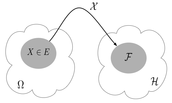
Figure 6.1.1: An RP maps the sample space $\Omega$ to a space $\mathcal{H}$ of functions from $J$ to $\R$. Given a set of functions $\mathcal{F}\subset\mathcal{H}$, the set $\mathcal{X}\in\mathcal{F}$ is the event $\{\omega\in\Omega: \mathcal{X}(\omega)\in\mathcal{F}\}\subset\Omega$.
Example 6.1.1.
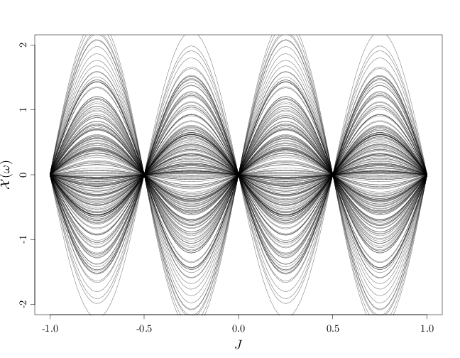
The process $\{X_t:t\in\R\}$ with $\Omega=\R$ and $X_t(\omega)=\omega \sin(2\pi t)$ is a continuous-time RP whose sample paths are sinusoidal curves amplified by $\omega\in\R$. If $\omega\sim N(0,\sigma^2)$ then sample paths with small amplitude are more probable than sample paths with large amplitude. The variables $X_t,X_{t'}$ are highly dependent and are in fact functions of each other: $X_t=f(X_{t'})$. For example, we have
\[ \P\left(\mathcal{X}\in\left\{f:\sup_{t\in\R} |f(t)|\leq 3\right\}\right) = \P(|\omega|\leq 3) = \frac{1}{\sqrt{2\pi}} \int_{-3}^3 e^{-z^2/2}\,dz.\]
(Note that the probability on the right hand side above is the probability of the RP taking values in set of functions.)
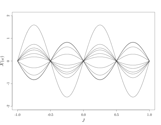
The following R code displays 10 and then 200 sample paths. The latter graph uses semi-transparent curves to demonstrate the higher density of sample paths near the $y=0$ axis.
par(cex.main = 1.5, cex.axis = 1.2, cex.lab = 1.5)
x = seq(-1, 1, length = 100)
A = sin(2 * pi * x) %*% t(rnorm(200))
plot(c(-1, 1), c(-2, 2), type = "n", xlab = "$J$",
    ylab = "$\\mathcal{X}(\\omega)$")
for (i in 1:10) lines(x, A[, i])
plot(c(-1, 1), c(-2, 2), type = "n", xlab = "$J$",
    ylab = "$\\mathcal{X}(\\omega)$")
for (i in 1:200) lines(x, A[, i], col = rgb(0, 0, 0,
    alpha = 0.5))