3.2. The Binomial Distribution

The Binomial RV, $X\sim\text{Bin}(n,\theta)$, where $\theta\in[0,1], n\in\mathbb{N}\cup\{0\}$, counts the number of successes in $n$ independent Bernoulli experiments with parameter $\theta$, regardless of the ordering of the results of the experiments.

If ordering does matter, the probability of particular sequence of $n$ experiments with $x$ successes and $n-x$ failures is $\theta^x(1-\theta)^{n-x}$. There are $n$-choose-$x$ such sequences, implying that \[ p_X(x)=\begin{cases}\left( \begin{array}{c} n \\ x \\ \end{array}\right) \theta^x (1-\theta)^{n-x} & x=0,1,\ldots,n\\ 0 & \text{otherwise} \end{cases}.\]

The fact that $P(X\in\Omega)=\sum_{x=0}^n p_X(x)=1$ may be ascertained using the binomial theorem (see Section 1.6): \begin{align*} 1=1^n=(\theta+(1-\theta))^n = \sum_{k=0}^n \left( \begin{array}{c} n \\ k \\ \end{array}\right) \theta^k(1-\theta)^{n-k}. \end{align*}

The binomial and Bernoulli RVs are closely related. A $\text{Ber}(\theta)$ RV has the same distribution as a $\text{Bin}(1,\theta)$ RV. On the other hand, a $\text{Bin}(n,\theta)$ RV is a sum of $n$ independent Bernoulli RVs $\text{Ber}(\theta)$. In the next chapter we show that if $Z^{(1)},\ldots,Z^{(n)}$ are RVs corresponding to independent experiments, then $\E(\sum Z^{(i)})=\sum \E Z^{(i)}$ and $\Var(\sum Z^{(i)})=\sum \Var(Z^{(i)})$. Using this result and the expectation and variance formulas of the Bernoulli RV, we derive that for $X\sim\text{Bin}(n,\theta)$ \begin{align*} \E(X) &= n\theta\\ \Var(X)&= n\theta(1-\theta). \end{align*}

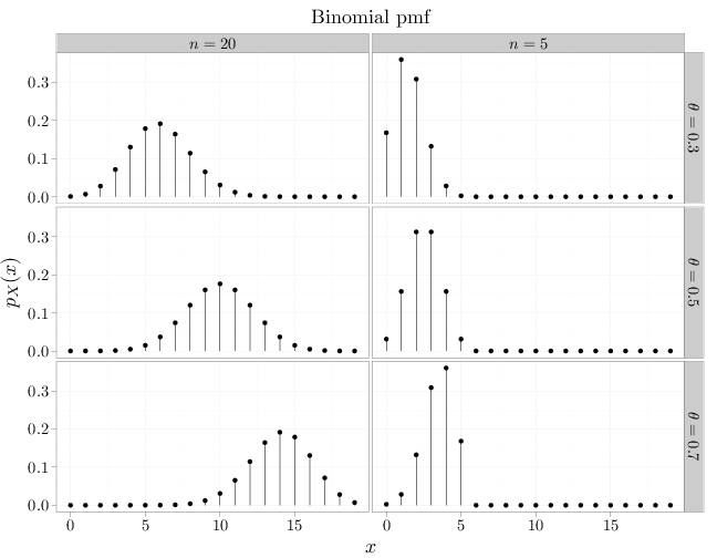
The formulas above indicate the following trends: as $\theta$ and $n$ increase the expectation increase, and as $n$ increases the variance increases. For a fixed $n$, the highest variance \[\max_{\theta\in[0,1]} \Var(X) = \max_{\theta\in[0,1]} n\theta(1-\theta)=n\max_{\theta\in[0,1]}(\theta-\theta^2)\] is obtained when $\theta=0.5$ (this can be verified by solving $0=(\theta-\theta^2)'=1-2\theta$ for $\theta$). This is in agreement with our intuition that an unbiased coin flip has more uncertainty than a biased coin flip. The R code below graphs the pmf of nine binomial distributions with different $n$ and $\theta$ parameters. The trends in the figure are in agreement with the observations above.

x = 0:19  # range of values to display in plot
# dbinom(x,n,theta) computes the pmf of
# Bin(n,theta) at x
y1 = dbinom(x, 5, 0.3)
y2 = dbinom(x, 5, 0.5)
y3 = dbinom(x, 5, 0.7)
y4 = dbinom(x, 20, 0.3)
y5 = dbinom(x, 20, 0.5)
y6 = dbinom(x, 20, 0.7)
D = data.frame(mass = c(y1, y2, y3, y4, y5, y6), x = x,
    n = 0, theta = 0)
D$n[1:60] = "$n=5$"
D$n[61:120] = "$n=20$"
D$theta[c(1:20, 61:80)] = "$\\theta=0.3$"
D$theta[c(21:40, 81:100)] = "$\\theta=0.5$"
D$theta[c(41:60, 101:120)] = "$\\theta=0.7$"
qplot(x, mass, data = D, main = "Binomial pmf", geom = "point",
    stat = "identity", facets = theta ~ n, xlab = "$x$",
    ylab = "$p_X(x)$") + geom_linerange(aes(x = x,
    ymin = 0, ymax = mass))