5.1. The Multinomial Random Vector

The two most important random vectors are the multinomial (discrete) and the multivariate Gaussian (continuous). The first generalizes the binomial random variable and the second generalizes the Gaussian random variable. This chapter describes both distributions, and concludes with a discussion of three more important random vectors: Dirichlet, mixtures, and the exponential family random vectors.

Since $\mathbb{P}_k$ is a set of points a linear constraint $\sum z_i=1$, $\mathbb{P}_k$ is a part of a $k-1$ dimensional linear hyperplane in $\R^{k}$. Figure 5.1.1 illustrates the spatial relationship between $\mathbb{P}_k$ and $\R^k$ for $k=3$.

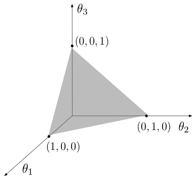
As described in Section 1.2, a probability function over a finite sample space $\Omega=\{\omega_1,\ldots,\omega_k\}$ is characterized by a vector of probability values $\bb{\theta}=(\theta_1,\ldots,\theta_k)$ satisfying $\theta_i\geq 0, i=1,\ldots,k$ and $\sum\theta_i=1$. The probability function is defined by the following equation \[\P(A)=\sum_{i\in A} \theta_i.\] This implies that the simplex $\mathbb{P}_k$ parameterizes the set of all distributions on a sample size $\Omega$ of size $k$. There exists a one-to-one and onto function mapping each elements of the simplex to distinct distributions.

We make the following comments.

1. The multivariate Bernoulli random vector is a unit vector describing the outcome of a random experiment with $k$ possible outcome - each outcome occurring with probability $\theta_k$.
2. Since $X_i=1$ implies $X_j=0$ for $j\neq i$, the multivariate Bernoulli random vector does not have independent components.
3. The pmf of a Bernoulli random vector may be written as \[ p_{\bb{X}}(\bb{x}) = \begin{cases} \prod_{i=1}^k \theta_i^{x_i} & \bb x \text{ is a unit vector}\\ 0 & \text{otherwise}\end{cases}.\]

The expectation vector and variance matrix (see Chapter 4) of the multivariate Bernoulli random vector are \begin{align*} \E(\bb{X})&=\bb{\theta}\\ \Var(\bb{X})&=\E(\bb{X}\bb{X}^{\top})-\E(\bb{X})\E(\bb{X})^{\top} = \text{diag}(\bb{\theta})-\bb{\theta}\bb{\theta}^{\top} \end{align*} where $\text{diag}(\bb{\theta})$ is a diagonal matrix with $(\theta_1,\ldots,\theta_k)$ as its diagonal (and 0 elsewhere). The derivations above follow from the fact that an expectation of a binary random variable is the probability of it being one.

We make the following observations.

1. Recall from Proposition 1.6.7 that the number of possible sequences of $N$ multivariate Bernoulli experiments resulting in $x_i$ successes in experiment $i$ for $i=1,\ldots,k$ is $N! / (x_1!\cdots x_k!)$ (where $N=\sum x_i$). It follows that the pmf of the multinomial random vector is \begin{align*} p_{\bb{X}}(\bb{x})= \begin{cases}\frac{N!}{x_1!\cdots x_k!} \theta_1^{x_1}\cdots\theta_k^{x_k} & x_i\geq 0,\,\, i=1,\ldots,k, \,\,\sum_{i=1}^k x_i=N\\ 0 & \text{otherwise} \end{cases}. \end{align*}
2. As in the case of the multivariate Bernoulli vector, the multinomial vector does not have independent components.
3. Since the multinomial random vector is a sum of independent multivariate Bernoulli random vectors, its expectation vector and variance matrix are (see Proposition 4.6.3 and Corollary 4.6.2) \begin{align*} \E(\bb{X})&=N\bb{\theta}\\ \Var(\bb{X})&= N\text{diag}(\bb{\theta})-N\bb{\theta}\bb{\theta}^{\top}. \end{align*}
4. The support of the multinomial pmf (the set of vectors $\bb x$ for which $p_{\bb X}(\bb x)>0$) satisfies a linear constraint $\sum x_i=N$, indicating that it lies on a $k-1$ dimensional linear hyperplane in $\R^k$.

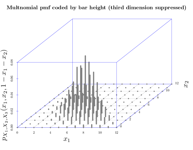
The following two graphs illustrate the multinomial pmf corresponding to $N=12$, and $\bb\theta=(0.5,0.3,0.2)$. The first graphs the pmf as a three dimensional bar chart, where the height of each bar indicates the probability or pmf value, and the two dimensional position of each bar corresponds to the vector ($x_1$, $x_2$). The third dimension is redundant since the three components of $\bb x$ have to sum to one. It appears that the multinomial pmf has a unimodal shape with the peak around the expectation vector $(6, 3.6, 2.4)$ (the peak in the graph is located at the first two components of the expectation vector).

library(scatterplot3d)
R = expand.grid(0:12, 0:12)
R[, 3] = 12 - R[, 1] - R[, 2]
names(R) = c("x1", "x2", "x3")
for (i in 1:nrow(R)) {
    v = R[i, 1:3]
    if (sum(v) == 12 & all(v >= 0)) {
        R$p[i] = dmultinom(v, prob = c(0.5, 0.3, 0.2))
    } else R$p[i] = 0
}
par(cex.main = 1.5, cex.axis = 1.2, cex.lab = 2, cex.symbols = 2,
    col.axis = "blue", col.grid = "lightblue")
scatterplot3d(x = R$x1, y = R$x2, z = R$p, type = "h",
    lwd = 10, pch = " ", xlab = "$x_1$", ylab = "$x_2$",
    zlab = "$p_{X_1,X_2,X_3}(x_1,x_2,1-x_1-x_2)$",
    color = grey(1/2))
title("Multnomial pmf coded by bar height (third dimension suppressed)")

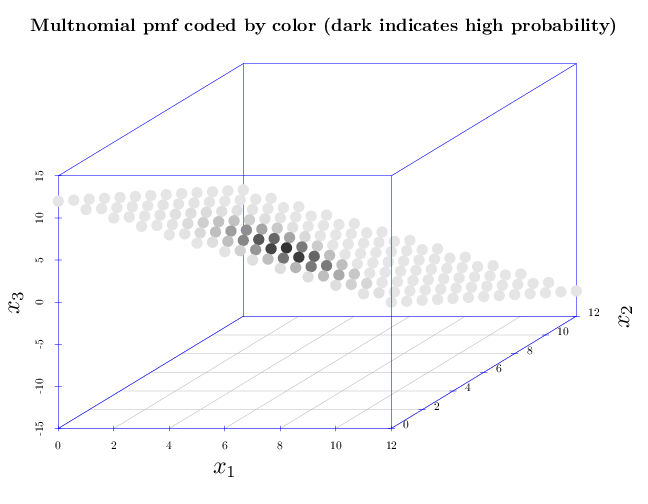
The second graph shows the non-negative values of the pmf using a three dimensional scatter plot. The three dimensions of each point correspond to its components $(x_1,x_2,x_3)$ and its gray level corresponds to its pmf $p_X(\bb x)$. The colors are assigned in the following manner: light gray colors correspond to high probabilities while dark gray colors correspond to low probabilities. It appears that the multinomial pmf is non-zero over a linear hyperplane, and has unimodal shape with the peak around the expectation vector $(6, 3.6, 2.4)$.

par(cex.main = 1.5, cex.axis = 1.2, cex.lab = 2, col.axis = "blue",
    col.grid = "lightblue")
scatterplot3d(x = R$x1, y = R$x2, z = R$x3, color = gray(0.9 -
    R$p * 10), type = "p", xlab = "$x_1$", pch = 16,
    ylab = "$x_2$", zlab = "$x_3$", cex.symbol = 2.5)
title("Multnomial pmf coded by color (dark indicates high probability)")