Probability
The Analysis of Data, volume 1
Important Random Variables: The Gamma and Chi-Squared Distributions
$
\def\P{\mathsf{\sf P}}
\def\E{\mathsf{\sf E}}
\def\Var{\mathsf{\sf Var}}
\def\Cov{\mathsf{\sf Cov}}
\def\std{\mathsf{\sf std}}
\def\Cor{\mathsf{\sf Cor}}
\def\R{\mathbb{R}}
\def\c{\,|\,}
\def\bb{\boldsymbol}
\def\diag{\mathsf{\sf diag}}
$
3.10. The Gamma and $\chi^2$ Distributions
Definition 3.10.1.
The gamma function is
\[ \Gamma(x) =\int_0^{\infty} t^{x-1}\exp(-t)\, dt, \qquad x>0.\]
Example F.2.5 shows, using integration by parts, that $\Gamma(n)=(n-1)!$ for positive integers $n$. The gamma function, however, is also defined for real numbers that are not integers.
Definition 3.10.2.
The gamma RV, $X\sim \text{Gam}(k,\theta)$, where $k,\theta\geq 0$, has the following pdf:
\begin{align}
f_X(x) = \begin{cases} x^{k-1} \theta^{-k} \exp(-x/\theta)/\Gamma(k) & x,k,\theta\geq 0\\ 0 &\text{otherwise}\end{cases}.
\end{align}
The gamma function in the denominator of the pdf ensures that the pdf integrates to 1:
\begin{align}
\int_0^{\infty} x^{k-1} \exp(-x/\theta)\,dx=
\theta\theta^{k-1} \int_0^{\infty} z^{k-1} \exp(-z)\,dz = \theta^k\Gamma(k).
\end{align}
Proposition 3.10.1.
The mgf of the gamma distribution is
$m(t) = (1-\theta t)^{-k}$, for $ t <1/\theta$.
Proof.
Defining $y=(1/\theta-t)x$,
\begin{align*}
m(t) &= \E(\exp(tX)) = \int_0^{\infty} x^{k-1} \frac{\exp(-x/\theta)}{\Gamma(k)\theta^k}\exp(tx) \, dx
\\&=\frac{1}{\Gamma(k)\theta^k} \int_0^{\infty} \left(\frac{y}{1/\theta-t} \right)^{k-1} \exp(-y) \, dy \frac{1}{1/\theta-t}\\
&=\frac{1}{\Gamma(k) (\theta(1/\theta-t)^{k}} \int_0^{\infty} y^{k-1}\exp(-y) \, dy = \left(1-\theta t\right)^{-k}.
\end{align*}
Proposition 3.10.2.
If $X_i\sim \text{Gam}(k_i,\theta)$, $i=1m\ldots,n$ are independent RVs, then
\[ \sum_{i=1}^n X_i \,\sim\, \text{Gam}\left(\sum_{i=1}^n k_i,\theta\right).\]
Proof.
This follows from the fact that the mgf of a sum of RVs is the product of their mgfs: $\prod (1-\theta t)^{-k_i}=(1-\theta t)^{\sum k_i}$.
Using the mgf, we can compute the expectation and variance of $X\sim \text{Gam}(k,\theta)$:
\begin{align*}
\E(X) &=m'(0) = k\theta (1-\theta t)^{-k-1}\Big |_{t=0} =k\theta\\
\E(X^2) &= m''(0)= k\theta (-k-1)(1-\theta t)^{-k-2}\Big |_{t=0}(-\theta)=k\theta^2(k+1) \\
\Var(X) &= k\theta^2(k+1) = k^2\theta^2= k\theta^2.
\end{align*}
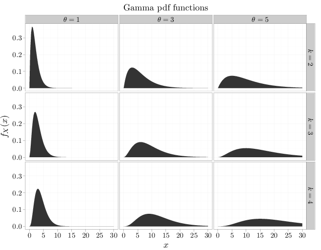
The non-constant parts of the pdf above (the parts that depend on $x$) include two multiplied terms: a decaying exponential $\exp(-x/\theta)$ and a polynomial $x^{k-1}$. As $x$ increases, the polynomial term is monotonic increasing and the exponential term is monotonic decreasing. For large $x$ the exponential decay is stronger than the polynomial growth (see Section B.5), implying that the pdf may be monotonic increasing for a while, but eventually decays to zero as $x\to\infty$. The shape of the pdf is generally unimodal, as in the case of the Gaussian distribution. Since the support is $[0,\infty)$, the pdf is necessarily asymmetric.
The R code below graphs the pdf of multiple gamma RVs with different parameter values.
x = seq(0, 30, length = 100)
y1 = dgamma(x, 2, scale = 1)
y2 = dgamma(x, 2, scale = 3)
y3 = dgamma(x, 2, scale = 5)
y4 = dgamma(x, 3, scale = 1)
y5 = dgamma(x, 3, scale = 3)
y6 = dgamma(x, 3, scale = 5)
y7 = dgamma(x, 4, scale = 1)
y8 = dgamma(x, 4, scale = 3)
y9 = dgamma(x, 4, scale = 5)
D = data.frame(probability = c(y1, y2, y3, y4, y5,
    y6, y7, y8, y9))
D$x = x
D$k[1:300] = "$k=2$"
D$k[301:600] = "$k=3$"
D$k[601:900] = "$k=4$"
D$theta[1:100] = "$\\theta=1$"
D$theta[101:200] = "$\\theta=3$"
D$theta[201:300] = "$\\theta=5$"
D$theta[301:400] = "$\\theta=1$"
D$theta[401:500] = "$\\theta=3$"
D$theta[501:600] = "$\\theta=5$"
D$theta[601:700] = "$\\theta=1$"
D$theta[701:800] = "$\\theta=3$"
D$theta[801:900] = "$\\theta=5$"
qplot(x, probability, data = D, geom = "area", facets = k ~
    theta, xlab = "$x$", ylab = "$f_X(x)$", main = "Gamma pdf functions")
Definition 3.10.3.
The chi-squared RV, $X\sim\chi^2_r$, where $r\in\mathbb{N}$, is a gamma RV with parameters
$k=r/2,\theta=2$. The parameter $r$ is called the degrees of freedom.
Corollary 3.10.1.
The mgf of the chi-squared distribution $\chi^2_r$ is $m(t)=(1-2t)^{-r/2}$.
The primary motivation of the chi-squared distribution is the following observation.
Proposition 3.10.2.
If $Z^{(1)},\ldots,Z^{(n)}$ are independent $N(0,1)$ RVs then
\[\sum_{i=1}^n (Z^{(i)})^2\,\,\sim\,\,\chi^2_n.\]
Proof.
Consider first the case $n=1$. The mgf of $(Z^{(1)})^2$ is
\begin{align*}
\E\left(e^{tZ^2}\right) &= \int_{-\infty}^{+\infty} e^{tz^2}
(2\pi)^{-1/2} e^{-z^2/2} dz = \int_{-\infty}^{+\infty} (2\pi)^{-1/2}
e^{-(1-2t)z^2/2} dz \\&= \frac{1}{(1-2t)^{1/2}}
\int_{-\infty}^{+\infty} \frac{e^{-z^2/(2(1-2t)^{-1})}}{\sqrt{2\pi}
(1-2t)^{-1/2}} dz = \frac{1}{(1-2t)^{1/2}} \cdot 1
\end{align*}
which is the mgf of $\chi^2_1$. In the case $n>1$, the mgf of the
sum is the product of $n$ mgfs of chi-squared RVs with one degree of freedom (see Proposition 4.8.1). This product is $\prod_{i=1}^n(1-2t)^{-1/2}=(1-2t)^{-n/2}$, which is the mgf of a $\chi^2_r$ RV.