5.2. The Multivariate Normal Vector

We make the following observations.

1. As Example C.1.2 shows, we have \[ f_{\bb{X}}(\bb{x}) = C(\bb\mu,\Sigma)\exp\left(-\frac{1}{2}\sum_{i=1}^n\sum_{j=1}^n (x_i-\mu_i)[\Sigma^{-1}]_{ij}(x_j-\mu_j)\right)\] where $C^{-1}=(2\pi)^{n/2}\sqrt{\det \Sigma}$ is constant in $\bb x$. This implies that the pdf decreases as the value of the quadratic form $\sum_{i=1}^n\sum_{j=1}^n (x_i-\mu_i)[\Sigma^{-1}]_{ij}(x_j-\mu_j)$ increases.
2. In the one dimensional case $n=1$, $\Sigma$ is a scalar, $\Sigma^{-1}=1/\Sigma$, and the pdf above reduces to the Gaussian RV pdf defined in Chapter 2.
3. Since the determinant of a symmetric positive definite matrix is positive (see Section 6.4), the square root of the determinant is a well defined positive real number.
4. The fact that the density integrates to 1 can be ascertained by the following change of variables \begin{align*} \bb{y}=\Sigma^{-1/2}(\bb{x}-\bb{\mu}),\qquad \bb{x}=\Sigma^{1/2}\bb{y}+\bb{\mu}. \end{align*} (see Proposition C.4.6 for a definition of the square root matrix $A^{1/2}$ of a given symmetric positive definite $A$) with a Jacobian determinant $|J|=\det(\Sigma^{1/2})=(\det\Sigma)^{1/2}$. Using Proposition F.6.3, we have \begin{align*} \int \exp\left(-\frac{1}{2}(\bb{x}-\bb{\mu})^{\top}\Sigma^{-1} (\bb{x}-\bb{\mu})\right)\, d\bb{x}&=\int \exp\left(-\frac{1}{2}\bb{y}^{\top}\Sigma^{1/2}\Sigma^{-1} \Sigma^{1/2}\bb{y}\right)\, |J|d\bb{y}\\ &=\int \exp\left(-\frac{1}{2}\bb{y}^{\top} \bb{y}\right)\, |J|d\bb{y}\\ &= |J| \prod_{j=1}^n\int \exp\left(-\frac{1}{2} y_j^2\right) \, dy_j \\ &= |J| \left((2\pi)^{1/2}\right)^n\\ &= (2\pi)^{n/2} (\det \Sigma)^{1/2} \end{align*} where the second-to-last equality follows from Example F.6.1. \end{itemize}
   Proposition 5.2.1. If $\bb{X}\sim N(\bb \mu,\Sigma)$ then \begin{align*} \Sigma^{-1/2}(\bb{X}-\bb{\mu})&\sim N(\bb 0,I)\\ \E(\bb{X})&=\bb{\mu} \\ \Var(\bb{X})&=\Sigma \end{align*}
   Proof. Using the change of variables $\bb{Y}=\Sigma^{-1/2}(\bb{X}-\bb{\mu})$ and derivations similar to observation 4 above, we have \begin{align*} f_{\bb{Y}}(\bb{y}) &= f_{\bb{X}}(\Sigma^{1/2}\bb y+\bb \mu) \,|J| \\ &= \frac{\sqrt{\det(\Sigma)}}{(2\pi)^{n/2}\sqrt{\det(\Sigma)}} \exp(-{\bb y}^{\top}\Sigma^{1/2}\Sigma^{-1}\Sigma^{1/2}\bb y ) \\ &= \prod_{j=1}^n \frac{1}{\sqrt{2\pi}} e^{-y_i^2} \end{align*} implying that $(Y_1,\ldots,Y_n)$ are mutually independent $N(0,1)$ RVs. \begin{align*} \E(\bb{X}) &= \E(\Sigma^{1/2}\bb Y+\bb{\mu})=\Sigma^{1/2}\E(\bb Y)+\bb{\mu} = \bb 0+\bb{\mu}\\ \Var(\bb{X}) &= \Var(\Sigma^{1/2}\bb{Y}+\bb{\mu}) = \Var(\Sigma^{1/2}\bb{Y})= (\Sigma^{1/2})^{\top}\Var(\bb{Y})\Sigma^{1/2}= (\Sigma^{1/2})^{\top}I\Sigma^{1/2}\\ &=\Sigma. \end{align*} Above, we used the fact that $\Sigma^{1/2}$ is symmetric and Corollary 4.6.3.

   The transformation $\bb{Y}=\Sigma^{-1/2}(\bb{X}-\bb{\mu})$ implies that if $X_1,\ldots,X_n$ are Gaussian RVs that are uncorrelated, or in other words $\Var(\bb{X})=I$, they are also independent. This is in contrast to the general case where a lack of correlation or $\Var(\bb X)=I$ does not necessarily imply independence.

   Proposition 5.2.2. If $X_i\sim N(\mu_i,\sigma_i), i=1,\ldots,n$ are independent RVs then \[{\bb a}^{\top}\bb X = \sum_{i=1}^n a_iX_i\sim N\left(\sum_{i=1}^n a_i\mu_i,\sum_{i=1}^n a_i^2\sigma_i^2\right), \qquad \bb a\in\R^n.\]
   Proof. Since the mgf of $N(\mu,\sigma^2)$ (see Section 3.9) is $e^{\mu t+\sigma^2 t^2/2}$, the mgf of $a_i X_i$ is $\E(\exp(t a_iX_i))$, which is the mgf of $X_i$ at $t a_i$: $e^{\mu t a_i+\sigma_i^2 t^2a_i^2/2}$. This is also the mgf of $N(a_i\mu,a_i^2\sigma_i^2)$, and by Proposition 2.4.2 this means that $a_iX_i\sim N(a_i\mu,a_i^2\sigma_i^2)$. Finally, from Proposition 4.8.1, \begin{align*} \prod_i e^{\mu t a_i+\sigma^2 t^2a_i^2/2} = e^{\sum_i \mu t a_i+\sigma_i^2 t^2a_i^2/2} = e^{t (\sum_i \mu a_i)+t^2(\sum \sigma_i^2 a_i^2)/2} \end{align*} which is the mgf of $N(\sum a_i\mu_i,\sum a_i^2\sigma_i^2)$. Using Proposition 2.4.2 again concludes the proof.
   Proposition 5.2.3. The multivariate mgf of $\bb X\sim N(\bb \mu,\Sigma)$ is \[ \E(\exp({\bb t}^{\top} \bb X)) = \exp\left({\bb t}^{\top} \bb \mu+{\bb t}^{\top}\Sigma\bb t /2\right).\]
   Proof. The mgf of $\bb Y\sim N(\bb 0,I)$ is \begin{align*} \E(\exp({\bb t}^{\top} \bb Y)) &= \E\left(\exp\left(\sum_{i=1}^n t_i Y_i \right)\right) \\ &= \E\left(\prod_{i=1}^n \exp\left( t_i Y_i \right)\right) \\ &= \prod_{i=1}^n \E\left( \exp\left( t_i Y_i \right)\right) \\ &= \exp\left({\bb t}^{\top}\bb t/2\right). \end{align*} Since $\bb X=\Sigma^{1/2}\bb Y+\bb \mu$, we use the transformation $\bb u=\Sigma^{1/2}\bb t$ to get \begin{align*} \E(\exp({\bb t}^{\top} \bb X)) &= \E\left(\exp\left({\bb t}^{\top}(\Sigma^{1/2}\bb Y+\bb \mu) \right)\right) \\ &= \E \left( \exp((\Sigma^{1/2}\bb t)^{\top}\bb Y)\right) \exp({\bb t}^{\top}\bb \mu)\\ &= \E \left(\exp(\bb u^{\top}\bb Y)\right) \E \exp({\bb t}^{\top}\bb \mu) \\ &= \exp\left({\bb u}^{\top}\bb u/2\right) \exp({\bb t}^{\top}\bb \mu) \\ &= \exp\left((\Sigma^{1/2}\bb t)^{\top} (\Sigma^{1/2}\bb t) /2\right) \exp({\bb t}^{\top}\bb \mu) \\ &=\exp (\bb t^{\top} \Sigma \bb t /2+ {\bb t}^{\top}\bb \mu). \end{align*}

   The proposition below shows that any affine transformation of a Gaussian random vector is also a Gaussian vector.

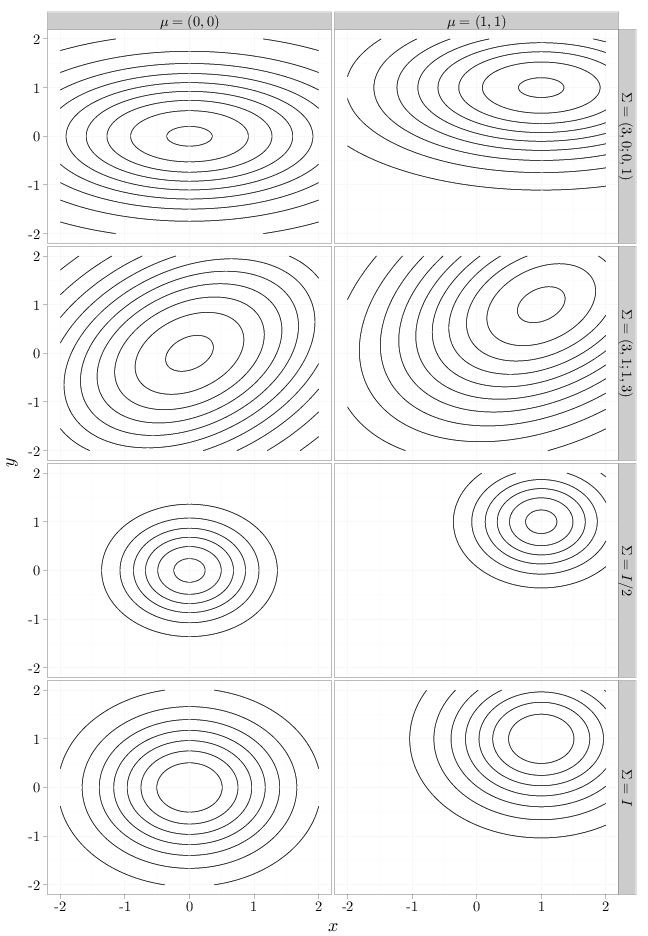
   Proposition 5.2.4. If $\bb X\sim N(\bb \mu,\Sigma)$ and $A$ is a matrix of full rank then \[A\bb X+\bb \tau \sim N(A\bb \mu+\bb \tau,A^{\top}\Sigma A).\]
   Proof. Using the transformation $\bb u=A^{\top} \bb t$, \begin{align*} \E \exp({\bb t}^{\top}( A\bb X+\bb \tau)) &= \left(\E \exp( (A^{\top}\bb t)^{\top}\bb X \right) \exp({\bb t}^{\top}\bb \tau) \\ &= \E (\exp( {\bb u}^{\top} \bb X) )\, \exp({\bb t}^{\top}\bb \tau) \\ &= \exp (\bb u^{\top} \Sigma \bb u /2+ {\bb u}^{\top}\bb \mu) \exp({\bb t}^{\top}\bb \tau)\\ &= \exp ((A^{\top}\bb t)^{\top} \Sigma (A^{\top}\bb t) /2+ (A^{\top}\bb t)^{\top}\bb \mu + {\bb t}^{\top}\bb \tau)\\ &= \exp ({\bb t}^{\top} (A \Sigma A^{\top}) \bb t) /2+ {\bb t}^{\top}(A\bb \mu+\bb \tau)), \end{align*} which is the mgf of the $N(A\bb \mu+\bb \tau,A \Sigma A^{\top})$ distribution. The fact that $A$ is full rank is needed to ensure that $A \Sigma A^{\top}$ is positive definite (this is a required property for the variance of the multivariate Gaussian distribution).

   As shown in Chapter 3, Gaussian RVs have pdfs that resemble a bell-shaped curve centered at the expectation and whose spread corresponds to the variance. The Gaussian random vector has an $n$-dimension pdf whose contour lines resemble ellipsoids centered at $\bb \mu$ and whose shape is determined by $\Sigma$. Recall that the leading term in the Gaussian pdf is constant in $\bb x$, implying that it is sufficient to study the exponent in order to investigate the shape of the equal height contours of $f_{\bb X}$.

   1. If $\Sigma$ is the identity matrix, its determinant is 1, its inverse is the identity as well, and the exponent of the Gaussian pdf becomes $-\sum_{i=1}^n (x_i-\mu_i)^2/2$. This indicates that the pdf factors into the product of $n$ pdf functions of normal RVs, with means $\mu_i$ and variance $\sigma^2_i=1$. In this case, the contours have spherical symmetry.
   2. If $\Sigma$ is a diagonal matrix with elements $[\Sigma]_{ij}=\sigma_i^2$, then its inverse is a diagonal matrix with elements $[\Sigma^{-1}]_{ij}=1/\sigma_i^2$ and $\det\Sigma=\prod_i \sigma_i^2$. The exponent of the pdf factors into a sum, indicating that the pdf factors into a product of independent Gaussian RVs $X_i\sim N(\mu_i,\sigma_i^2), i=1,\ldots,n$. The equal height contours are axis-aligned ellipses, whose spread along each dimension depends on $\sigma_i^2$.
   3. In the general case, the exponent is $-\sum_i\sum_j(x_i-\mu_i)\Sigma_{ij}^{-1}(x_j-\mu_j)$, which is a quadratic form in $\bb x$. As a result, the equal height contours of the pdf will be elliptical with a center determined by $\bb{\mu}$ and shape determined by $\Sigma$. The precise relationship is investigated in Section C.3 (see also exercise 3 at the end of this chapter).

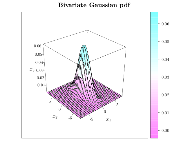
   The R code below graphs the pdf of a two dimensional Gaussian random vector with expectation $(0,0)$ and variance matrix $\begin{pmatrix} 1 & 0\\ 0 & 6\end{pmatrix}$.

   library(lattice)
   trellis.par.set(list(fontsize = list(text = 18)))
   R = expand.grid(seq(-8, 8, length = 30), seq(-8, 8,
       length = 30))
   names(R) = c("x1", "x2")
   R$p = dmvnorm(R, sigma = matrix(c(1, 0, 0, 6), nrow = 2,
       ncol = 2))
   wireframe(p ~ x1 + x2, data = R, xlab = "$x_1$", ylab = "$x_2$",
       zlab = "$x_3$", main = "Bivariate Gaussian pdf",
       scales = list(arrows = FALSE), drape = TRUE)
   

   

   The R code below graphs the equal height contours of eight two dimensional Gaussian pdfs with different $\mu$ and $\Sigma$ parameters. Note how modifying the $\mu$ parameter shifts the pdf and modifying $\Sigma$ changes the shape of the contour lines as described above.

   R = expand.grid(seq(-2, 2, length = 100), seq(-2, 2,
       length = 100))
   z1 = dmvnorm(R, c(0, 0), diag(2))
   z2 = dmvnorm(R, c(0, 0), diag(2)/2)
   z3 = dmvnorm(R, c(0, 0), matrix(c(3, 0, 0, 1), nrow = 2,
       ncol = 2))
   z4 = dmvnorm(R, c(0, 0), matrix(c(3, 1, 1, 3), nrow = 2,
       ncol = 2))
   z5 = dmvnorm(R, c(1, 1), diag(2))
   z6 = dmvnorm(R, c(1, 1), diag(2)/2)
   z7 = dmvnorm(R, c(1, 1), matrix(c(3, 0, 0, 1), nrow = 2,
       ncol = 2))
   z8 = dmvnorm(R, c(1, 1), matrix(c(3, 1, 1, 3), nrow = 2,
       ncol = 2))
   S1 = stack(list(`$\\Sigma=I$` = z1, `$\\Sigma=I/2$` = z2,
       `$\\Sigma=(3,0;0,1)$` = z3, `$\\Sigma=(3,1;1,3)$` = z4,
       `$\\Sigma=I$` = z5, `$\\Sigma=I/2$` = z6, `$\\Sigma=(3,0;0,1)$` = z7,
       `$\\Sigma=(3,1;1,3)$` = z8))
   S1$mu = "$\\mu=(0,0)$"
   S1$x = R[, 1]
   S1$y = R[, 2]
   S1$mu[1:40000] = "$\\mu=(0,0)$"
   S1$mu[40001:80000] = "$\\mu=(1,1)$"
   ggplot(S1, aes(x = x, y = y, z = values)) + xlab("$x$") +
       ylab("$y$") + facet_grid(ind ~ mu) + stat_contour()