3.13. Mixture Distribution

The distributions above have simple shape, in the sense that their pdf or pmf functions are constant, monotonic increasing or decreasing, or unimodal. This section and the next two sections describe methods of constructing distributions that are more complex, potentially having multiple local maxima and minima.

Given $k$ independent RVs $X^{(1)},\ldots,X^{(k)}$ that are all continuous or all discrete, their mixture is an RV with the following pdf or pmf \begin{align} f_{X}(x) &= \sum_{i=1}^k \alpha_i f_{X^{(i)}}(x) \qquad \text{(continuous case)}\\ p_{X}(x) &= \sum_{i=1}^k \alpha_i p_{X^{(i)}}(x) \qquad \text{(discrete case)}. \end{align} where $\bb\alpha=(\alpha_1,\ldots,\alpha_n)$ is a vector of non-negative numbers that sum to 1. Since the weights sum to one, the above functions are valid pdf or pmf and thus uniquely characterize the mixture distribution.

The moments of a mixture random variables are linear combinations of the corresponding moments of the individual random variables: \begin{align*} \E(X) = \sum_{i=1}^k \alpha_i \E(X^{(i)})\\ \Var(X) = \sum_{i=1}^k \alpha_i^2 \Var(X^{(i)}). \end{align*}

Mixture distributions are able to capture a wide variety of complex distributions. For example, a mixture of $k$ Gaussians can capture a distribution with $k$ modes. Mixture distributions are particularly applicable to situations when the quantity is determined via a two stage experiment: first a mixture component is chosen, and then the value is determined from the appropriate mixture component. For example, consider the situation of measuring with length of fish found in a certain lake containing $k$ species of fish. Assuming fish in different species have significantly different lengths, and that within each of the species the variability in length is limited, we have a mixture model with $k$ components: $X^{(i)}, i=1,\ldots,k$ represents the distribution of lengths among the species, and $\bb w$ represents the relative frequency of the different species.

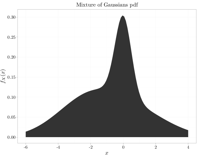
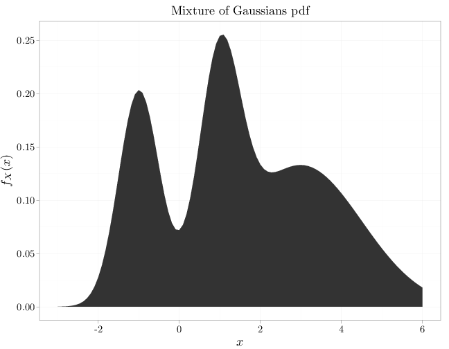
The R code below graphs two mixtures of three Gaussians. The first example exhibits a multimodal shape while the second exhibits a asymmetric unimodal shape.

x = seq(-3, 6, length = 100)
y1 = dnorm(x, -1, 1/2)
y2 = dnorm(x, 1, 1/2)
y3 = dnorm(x, 3, 1.5)
qplot(x, y1/4 + y2/4 + y3/2, xlab = "$x$", ylab = "$f_X(x)$",
    geom = "area", main = "Mixture of Gaussians pdf")

x = seq(-6, 4, length = 100)
y1 = dnorm(x, 1, 2)
y2 = dnorm(x, 0, 1/2)
y3 = dnorm(x, -2, 2)
qplot(x, y1/4 + y2/4 + y3/2, xlab = "$x$", ylab = "$f_X(x)$",
    geom = "area", main = "Mixture of Gaussians pdf")