3.15. The Smoothed Empirical Distribution

One difficulty with the empirical distribution is that it assigns positive probability mass only to a finite number of points, which may be undesirable when modeling continuous variables. The smoothed empirical distribution combines the ideas in the previous two sub-sections. Given a sequence of values $y^{(1)},\ldots,y^{(n)}$, $y^{(i)}\in\R$, the smoothed empirical distribution is defined as a mixture distribution with the following pdf \[f_X(x) = \frac{1}{n} \sum_{i=1}^n f_{\sigma}(x-y^{(i)}), \] where $f_{\sigma}$ is usually a symmetric unimodal pdf with expectation 0 and variance $\sigma^2$. The mixture pdf is thus a sum of pdfs $f_{\sigma}(x-y^{(1)}), \ldots, f_{\sigma}(x-y^{(n)})$ with variance $\sigma^2$ and centered at the values $y^{(1)},\ldots,y^{(n)}$.

A popular choice for $f_{\sigma}$ is the Gaussian pdf $N(0,\sigma^2)$. In this case, we have \[f_X(x) = \frac{1}{n\sqrt{2\pi\sigma^2}} \sum_{i=1}^n \exp\left( -(x-y^{(i)})^2/(2\sigma^2) \right).\] As $\sigma$ decreases, the smoothed empirical distribution converges to the empirical distribution. As $\sigma$ increases, the role of the individual mixtures decreases and the distribution approaches a single monolithic component.

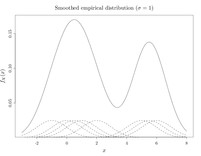
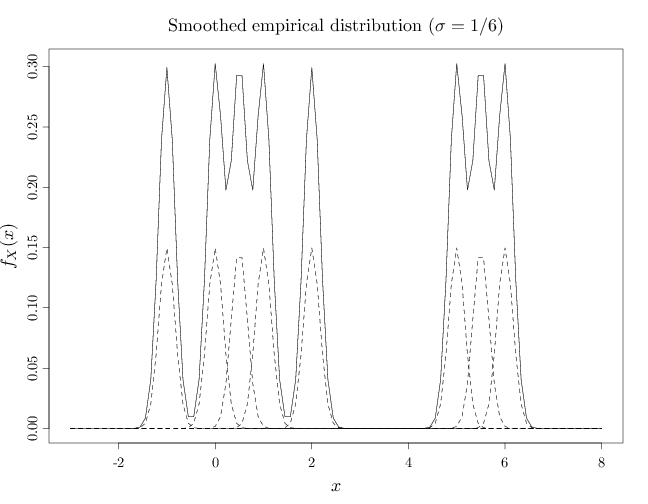
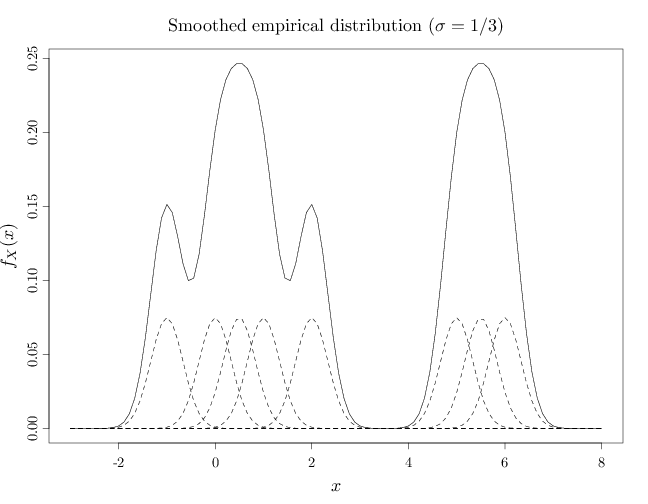
The R code below graphs the smoothed version of the empirical distribution corresponding to the sequence $(-1, 0, 0.5, 1, 2, 5, 5.5, 6)$. The graphs show the empirical distribution as a solid line and the mixture components $f_{\sigma}(x-y^{(i)})$, $i=1,\ldots,8$ corresponding to each $y^{(i)}$ with dashed lines (scaled down by a factor of 2 to avoid overlapping solid and dashed lines).

In the first graph below, the $\sigma$ value is relatively small ($\sigma=1/6$), resulting in a pdf close to the empirical distribution. In the middle case $\sigma$ is larger ($\sigma=1/3$) showing a multimodal shape that is significantly different from the empirical distribution. In the third case above, $\sigma$ is relatively large ($\sigma=1$), resulting in a pdf that is resembles two main components. For larger $\sigma$, the pdf will resemble a single monolithic component.

A = c(-1, 0, 0.5, 1, 2, 5, 5.5, 6)
x = seq(-3, 8, length.out = 100)
D = x %o% rep(1, 8)
f = x * 0
for (i in 1:8) {
    D[, i] = dnorm(x, A[i], 1/6)/8
    f = f + D[, i]
}
par(cex.main = 1.5, cex.axis = 1.2, cex.lab = 1.5)
plot(x, f, xlab = "$x$", ylab = "$f_X(x)$", type = "l")
for (i in 1:8) lines(x, D[, i]/2, lty = 2)
title("Smoothed empirical distribution ($\\sigma=1/6$)",
    font.main = 1)

A = c(-1, 0, 0.5, 1, 2, 5, 5.5, 6)
x = seq(-3, 8, length.out = 100)
D = x %o% rep(1, 8)
f = x * 0
for (i in 1:8) {
    D[, i] = dnorm(x, A[i], 1/3)/8
    f = f + D[, i]
}
plot(x, f, xlab = "$x$", ylab = "$f_X(x)$", type = "l")
for (i in 1:8) lines(x, D[, i]/2, lty = 2)
title("Smoothed empirical distribution ($\\sigma=1/3$)",
    font.main = 1)

A = c(-1, 0, 0.5, 1, 2, 5, 5.5, 6)
x = seq(-3, 8, length.out = 100)
D = x %o% rep(1, 8)
f = x * 0
for (i in 1:8) {
    D[, i] = dnorm(x, A[i], 1)/8
    f = f + D[, i]
}
plot(x, f, xlab = "$x$", ylab = "$f_X(x)$", type = "l")
for (i in 1:8) lines(x, D[, i]/2, lty = 2)
title("Smoothed empirical distribution ($\\sigma=1$)",
    font.main = 1)