7.3. Gaussian Processes
In order to invoke Kolmogorov's extension theorem and ensure the above definition is rigorous, we need the covariance function $C$ to (i) produce legitimate covariance matrices (symmetric positive definite matrices), and (ii) produce consistent finite dimensional marginals, in the sense of Definition 6.2.1. The second requirement of consistency of the finite dimensional marginals can be ensured by defining the covariance function to be \[[C({\bb t}_1,\ldots,{\bb t}_k))]_{ij} = C'({\bb t}_i,{\bb t}_j) \] for some function $C':\R^d\times \R^d\to\R$.
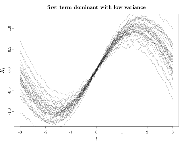
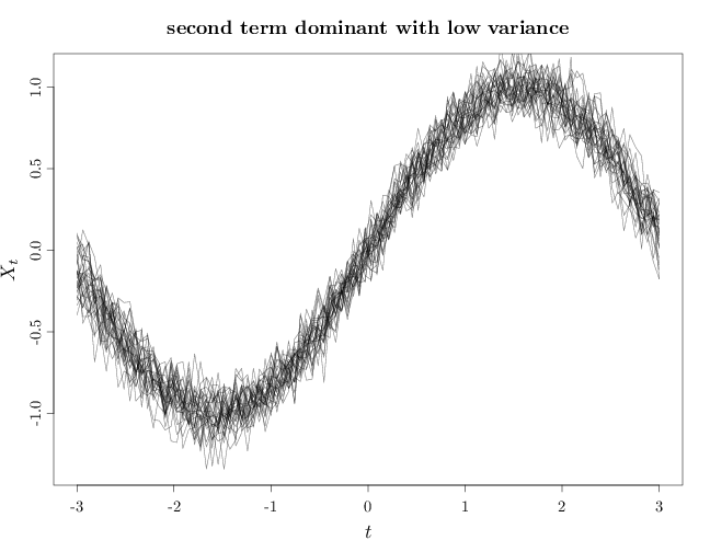
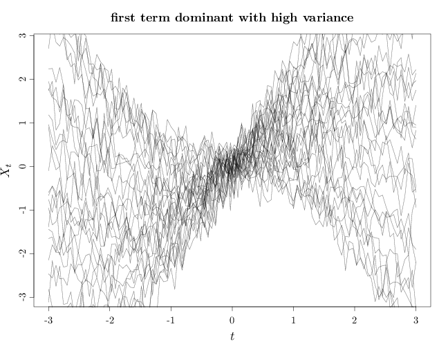
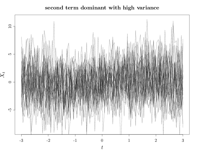
As $\alpha,\beta$ increase the variance increases making the process more likely to vary further from the expectation function $m$. If $\beta \ll \alpha$, the first term in the covariance function becomes dominant, implying that the variance grows similarly to $\langle {\bb t}_1, {\bb t}_2\langle$. If $d=1$, this means that $X_t,X_s$ are positively correlated if $t, s$ have the same sign and negatively correlated if $t, s$ have opposing signs. Furthermore, the degree of correlation in absolute value increases as $|t|,|s|$ increase. If $\alpha \ll \beta$ the second term in the covariance function becomes dominant, implying that as the process values at two distinct times ${\bb t}_1$, ${\bb t}_2$ is uncorrelated and therefore independent. The resulting process has marginals $X_{\bb t}, \bb t \in \R^k$ that are independent $N(m(\bb t), \beta)$ random variables.
The R code below graphs samples from this random process in four cases: first term dominant with low variance, second term dominant with low variance, first term dominant with high variance, and second term dominant with high variance. In all cases the expectation function is a sinusoidal curve $m(t)=\sin(t)$. Note that in general, the sample paths are not smooth curves.
X = seq(-3, 3, length.out = 100)
m = sin(X)
n = 30
I = diag(1, nrow = 100, ncol = 100)
Y1 = rmvnorm(n, m, X %o% X/100 + I/1000)
par(cex.main = 1.5, cex.axis = 1.2, cex.lab = 1.5)
plot(X, Y1[1, ], type = "n", xlab = "$t$", ylab = "$X_t$",
    main = "first term dominant with low variance")
for (s in 1:n) lines(X, Y1[s, ], col = rgb(0, 0, 0,
    alpha = 0.5))
Y2 = rmvnorm(n, m, X %o% X/1000 + I/100)
plot(X, Y2[1, ], type = "n", xlab = "$t$", ylab = "$X_t$",
    main = "second term dominant with low variance")
for (s in 1:n) lines(X, Y2[s, ], col = rgb(0, 0, 0,
    alpha = 0.5))
Y3 = rmvnorm(n, m, X %o% X + I/10)
plot(X, Y3[1, ], type = "n", xlab = "$t$", ylab = "$X_t$",
    main = "first term dominant with high variance")
for (s in 1:n) lines(X, Y3[s, ], col = rgb(0, 0, 0,
    alpha = 0.5))
Y4 = rmvnorm(n, m, X %o% X + I * 10)
plot(X, Y4[1, ], type = "n", xlab = "$t$", ylab = "$X_t$",
    main = "second term dominant with high variance")
for (s in 1:n) lines(X, Y4[s, ], col = rgb(0, 0, 0,
    alpha = 0.5))
The Wiener Process
An interesting special case of the Gaussian process is the Wiener process.
We motivate the Wiener process by deriving it informally as the limit of a discrete-time discrete-valued random walk process with step size $h$.
Let $Z_t=\sum_{i=1}^n h Y_n$, for some $h>0$, where $Y_n=2 X_n-1$ and $X_n\iid \text{Ber}(1/2), n\in \mathbb{N}$. Since $\E(Y_n)=\E(2X_n-1) = 2\cdot 1/2-1=0$ and $\Var(Y_n)=\Var(2X_n-1)=4\Var(X_n)=4(1/2)(1-1/2)=1$, we have $\E(hY_n) = 0$ and $\Var(hY_n) = h^2$.
We set $h=\sqrt{\alpha \delta}$ and let $\delta\to 0, h\to 0$, or alternatively $h=\sqrt{\alpha}\sqrt{t/n}$ and let $n\to\infty$. This yields \begin{align*} Z_t & = \lim_{n\to\infty} \sqrt{\alpha}\sqrt{t/n} \sum_{i=1}^n Y_n = \sqrt{\alpha t} \lim_{n\to\infty} \frac{\sum_{i=1}^n Y_n}{\sqrt{n}}. \end{align*} Intuitively, the segment $[0,t]$ is divided to $n$ steps of size $\delta=t/n$ each, and $Z_t$ measures the position of the symmetric random walk at time $t$ or equivalently after $n$ steps of size $\delta$. By the central limit theorem (see Section 8.9) $\lim_{n\to\infty} \sum_{i=1}^n Y_n / \sqrt{n}$ approaches a Gaussian RV with mean zero and variance one. Since $Z_t$ approaches $\sqrt{\alpha t}$ times a $N(0,1)$ RV, we have as $n\to\infty$ \[Z_t\sim N(0,\alpha t).\]
To show that the limit of the random walk above corresponds to Definition 7.3.2, it remains to show that (i) $\mathcal{Z}$ is a Gaussian process and (ii) it has a zero expectation function and its auto-covariance function is $C_{\mathcal{Z}}(t,s)=\alpha\min(t,s)$.
The increments of $\mathcal{Z}$ are independent and have the same distribution. For example $Z_5-Z_3$ is independent of $Z_2-Z_0=Z_2$ and have the same distribution. Since \[f_{Z_{t_1},\ldots,Z_{t_k}}(\bb{z})= f_{Z_{t_1}}(z_1) f_{Z_{t_2}-Z_{t_1}}(z_2-z_1)\cdots f_{Z_{t_{k}}-Z_{t_{k-1}}}(z_k-z_{k-1}), \] the pdf of a finite dimensional marginal $f_{Z_{t_1},\ldots,Z_{t_k}}$ is a product of independent univariate Gaussians, which has a multivariate Gaussian distribution.
The mean function $m_{\mathcal{Z}}(t)=0$ as it is a sum of zero mean random variables. The auto-covariance function is \begin{align*} C_{\mathcal{Z}}(t,s) &=\E\left(\left(\lim \sum_{i=1}^{ t/\delta } h Y_i\right)\left( \lim \sum_{i=1}^{s/\delta } h Y_i\right)\right) = \lim h^2 \E\left(\sum_{i=1}^{ t/\delta }\sum_{j=1}^{ s/\delta }Y_iY_j \right) \\ &= \lim h^2 \sum_{i=1}^{ t/\delta }\sum_{j=1}^{ s/\delta } \E(Y_iY_j) = \lim h^2 \sum_{i=1}^{\min(s,t)/\delta } \E(Y_i^2)\\ & =\lim h^2 \min(s,t)\Var(Y)/\delta = \lim \alpha\delta\min(s,t)/\delta \\ &=\alpha \min(s,t), \end{align*} where in the third equation above we used the fact that $\E(Y_iY_j)=0$ for $i\neq j$ (since $Y_i,Y_j$ are independent RVs with mean 0).