6.2. Random Processes and Marginal Distributions
Given a random process we can consider its finite dimensional marginals, namely the distribution of $X_{t_1},\ldots,X_{t_k}$ for some $k\in\mathbb{N}$ and some $t_1,\ldots,t_k\in J$. The marginals distributions are characterized by the corresponding joint cdf functions \[ F_{X_{t_1},\ldots,X_{t_k}}(r_1,\ldots,r_k) = \P(X_{t_1}\leq r_1,\ldots,X_{t_k}\leq r_k) \] where $k\geq 1$, $t_1,\ldots,t_k\in J$ and $r_1,\ldots,r_k\in\R$. If the process RVs are discrete, we can consider instead the joint pmf functions, and if the process RVs are continuous, we can consider instead the joint pdf functions.
Given an RP $\mathcal{X}=\{X_t:t\in J\}$, all finite dimensional marginals are defined. Kolmogorov's extension theorem below states that the reverse also holds: a collection of finite dimensional marginal distributions uniquely defines a random process, as long as the marginals do not contradict each other. Consequentially, we now have a systematic way to define random processes by defining a collection of all finite dimensional marginals (that are consistent with each other).
- If $F_{X_{t_1},\ldots,X_{t_k}}\in\mathcal{L}$ and $F_{X_{t_1},\ldots,X_{t_k},X_{t_{k+1}}}\in\mathcal{L}$ then for all $r_1,\ldots,r_{k+1}\in\R$ \begin{align*} F_{X_{t_1},\ldots,X_{t_k}}(r_1,\ldots,r_k) = \lim_{r_{k+1}\to+\infty} F_{X_{t_1},\ldots,X_{t_k},X_{t_{k+1}}}(r_1, \ldots,r_k, r_{k+1}). \end{align*}
- If $\mathcal{L}$ has two finite dimensional marginal cdfs over the same RVs, the order in which the RVs appear is immaterial; for example, \[ F_{X_{t_1},X_{t_2}}(r_1,r_2)=F_{X_{t_2},X_{t_1}}(r_2,r_1).\]
The finite dimensional marginals arising from a random process satisfy the consistency definition above since they are derived from the same joint distribution $\P$ over the common sample space $\Omega$. Kolmogorov's extension theorem below states that the converse also holds. The proof for discrete time RPs is available in Section 6.5. A proof for continuous time RPs is available in (Billingsley, 1995).
Instead of specifying a process by its finite dimensional marginal cdfs, we may do so using all finite dimensional marginal pdfs (if $X_t$, $t\in J$ are continuous) or all finite dimensional marginal pmfs (if $X_t$, $t\in J$ are discrete). In the former case, the first consistency condition in Definition 6.2.1 becomes \begin{align*} f_{X_{t_1},\ldots,X_{t_k}} (r_1,\ldots,r_k) = \int_{\R} f_{X_{t_1},X_{t_k},X_{t_{k+1}}} (r_1,\ldots,r_k,r_{k+1})\, dr_{k+1} \end{align*} and in the latter case, the condition becomes \begin{align*} p_{X_{t_1},\ldots,X_{t_k}} (r_1,\ldots,r_k) = \sum_{r_{k+1}} p_{X_{t_1},\ldots,X_{t_k},X_{t_{k+1}}} (r_1,\ldots,r_k,r_{k+1}). \end{align*}
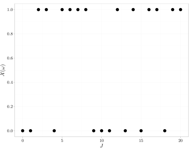
Note that the iid process above satisfies the consistency conditions, and as a result of Kolmogorov's extension theorem it characterizes a unique RP.
J = 0:20
X = rbinom(n = 21, size = 1, prob = 0.5)
qplot(x = J, y = X, geom = "point", size = I(5), xlab = "$J$",
    ylab = "$\\mathcal{X}(\\omega)$")
The examples we have considered thus far represent the two extreme cases: total independence in Example 6.2.2 and total dependence in Example 6.2.1 ($X_t$ is a function of $X_{t'}$ for all $t,t'\in J$). In general, the RVs $X_t$, $X_{t'}$ may be neither independent nor functions of each other.
Two important classes of random processes are stationary processes and Markov processes. They are defined below.
A process with independent increments is necessarily Markov, but the converse does not hold in general.