7.2. Poisson Process

The Poisson process is a continuous-time discrete-state Markov process $\{X_t: t\geq 0\}$ where $X_t\in\mathbb{N}$ counts the number of independent arrivals or events occurring in the time interval $[0,t]$. The Poisson process additionally assumes the following:

1. The probability of getting a single arrival or event in a small time interval $[t,t+\Delta]$ is $\Delta\cdot\lambda$, where $\lambda>0$ is commonly referred to as the intensity of the process.
2. The probability of getting more than a single event in a small time interval is negligible.

The Poisson process is often used to model the count of independent arrivals. Examples include arrivals of cars in an intersection and arrival of phone calls at a telephone switchboard. The Poisson process marginals $X_t$ are random variables counting the number of such arrivals in the time interval $[0,t]$.

We proceed with a more formal definition of the Poisson process, and follow with some properties.

7.2.1 Postulates and Differential Equation

The Poisson process is motivated by the following basic postulates:

1. The process $\{X_t:t\geq 0\}$ is a continuous time discrete state Markov process for which \[P_{ij}(t)\defeq \P(X_{t+u}=j \c X_{u}=i).\] Note specifically that $P_{ij}(t)$ does not depend on $u$.
2. \[\lim_{h\to 0} \P(X_{t+h}-X_t=1 \c X_{t}=x)/h=\lambda,\] or, alternatively using the growth notation (see Section B.5): \[\P(X_{t+h}-X_t=1 \c X_{t}=x)=\lambda h+ o(h).\]
3. $\P(X_0=0)=1$
4. $\P(X_{t+h}-X_t=0 \c X_{t}=x)=1-\lambda h+o(h)$.

Postulates 2 and 4 imply that the probability of multiple events occurring in a short time interval is negligible (formally, it decays to zero faster than the interval size). Thus, the distribution of the number of arrivals in a short time interval $[t,t+h]$ is approximately a Bernoulli distribution with parameter $\lambda h$.

Denoting $P_m(t)=\P(X_t=m)$, the above postulates imply \[P_0(t+h)=P_0(t)P_0(h)=P_0(t)(1-\lambda h+o(h)),\] which in turn imply \[(P_0(t+h)-P_0(t))/h=-P_0(t) (\lambda h+o(h))/h=-P_0(t) (\lambda +o(1)).\] This leads to the differential equation: \begin{align} \tag{*} P_0'(t)=-\lambda P_0(t). \end{align} Subject to the initial condition $X_0=0$ (postulate 3), the solution of the above equation is \begin{align*} P_0(t)=e^{-\lambda t}, \end{align*} as can be verified by substituting the solution above in (*). Using the law of total probability (Proposition 1.5.4), we get that, for some constant $C$, \begin{align*} P_m(t+h)-P_m(t) &= P_m(t)P_0(h)+P_{m-1}(t)P_1(h)+\sum_{j=2}^m P_{m-j}(t)P_j(h)-P_m(t)\\ &=P_m(t)(1-\lambda h + o(h))+P_{m-1}(t)(\lambda h +o(h)))+o(h)C-P_m(t)\\ &= -\lambda P_m(t) h + \lambda P_{m-1}(t)h + o(h), \end{align*} which leads to the following differential equation: \begin{align*} P_m'(t) &= \lim_{h\to 0} \frac{P_m(t+h)-P_m(t)}{h} =-\lambda P_m(t) + \lambda P_{m-1}(t). \end{align*}

The Poisson process is closely related to a number of important random variables, including the Poisson RV, the exponential RV, the binomial RV, and the uniform RV. We describe these relationships below.

7.2.2 Relationship to Poisson Distribution

Solving the differential equation above recursively for $P_m(t)$ using $P_0(t)=e^{-\lambda t}$ and $P_m(0)=0$ yields the solution \begin{align*} P_m(t)=\frac{\lambda^m t^m}{m!}\exp(-\lambda t), \end{align*} implying that \[X_t\sim \text{Poisson}(\lambda t), \qquad t\geq 0.\]

Alternatively, it is possible to verify the solution by by substituting it in the differential equation and verifying that equality holds.

Since a sum of independent Poisson RVs is a Poisson RV (see Section 3.6) the distribution of the number of events in the interval $[s,t]$ is \[ X_t - X_{s} \sim \text{Poisson}(\lambda(t-s)).\] Using the moments of the Poisson distribution (see Section 3.6), we get the following expressions for the mean and auto-covariance functions: \begin{align*} m(t) &= \lambda t\\ C(t,s) &=\E((X_s-\lambda s)(X_t-\lambda t)) =\E((X_s-\lambda s)((X_t-X_s-\lambda t+\lambda s) + (X_s-\lambda s)))\\ &=\Var(X_s) + \E((X_s-\lambda s)(X_t-X_s-\lambda t+\lambda s))\\ &=\Var(X_s)+\E(X_s-\lambda s)\E(X_t-X_s-\lambda t+\lambda s)\\ &=\Var(X_s) = \lambda s = \lambda\min(s,t). \end{align*} The equation above assumes $s\leq t$. A similar derivation holds in the case of $t\leq s$.

7.2.2 Relationship to Exponential Distribution

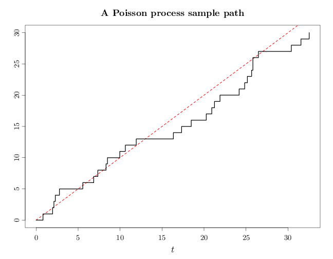
The code below shows a sample path of the Poisson process with $\lambda=1$ overlaid with the expectation function $m(t)=1\cdot t$. The generation of the sample path uses the proposition above by sampling the wait times and translating these values to the corresponding arrival times. Note how the arrivals represented by discontinuous jumps below occur at arbitrary $t$ values, rather than integers, demonstrating the continuous-time nature of the process.

Z = rexp(30, 1)
t = seq(0, sum(Z), length.out = 200)
X = t * 0
for (i in 1:30) {
    Zc = cumsum(Z)
    X[t >= Zc[i]] = i
}
par(cex.main = 1.5, cex.axis = 1.2, cex.lab = 1.5)
plot(c(0, sum(Z)), c(0, 30), type = "n", xlab = "$t$",
    ylab = "")
curve(x * 1, add = TRUE, col = rgb(1, 0, 0), lwd = 2,
    lty = 2, xlab = "$t$", ylab = "$X_t$")
lines(t, X, lwd = 3, type = "s")
title("A Poisson process sample path")

7.2.3 Relationship to Binomial Distribution

Recalling postulates 2 and 4 of the Poisson process, which imply that an arrival in $[h,h+\Delta]$ is approximately a Bernoulli RV (for small $\Delta$) with parameter $\lambda h$, we have that $X_t$ is approximately the sum of $t/\Delta$ independent Bernoulli RVs, and therefore is approximately a binomial RV. See also Section 3.6, which asserts that the binomial distribution with $n\to\infty$, $\theta\to 0$ and $n\theta\to\lambda$ is approximately a Poisson distribution.

Another relationship between the Poisson process and the binomial distribution is that for $u < t$ and $k < n$ \begin{align*} \P(X_u=k \c X_t=n) &= \frac{\P(X_u=k)\P(X_t-X_u=n-k)}{\P(X_t=n)}\\ &= \frac{\text{Pois}(k\,;\lambda u)\text{Pois}(n-k\,;\lambda(t-u))}{\text{Pois}(n,;\lambda t)}\\ &= \begin{pmatrix}n\\k\end{pmatrix} (u/t)^k (1-u/t)^{n-k} = \text{Bin}(k\,; n, u/t) . \end{align*} In other words, given $n$ arrivals by time $t$, the distribution of $k$ arrivals by time $u$ is binomial with parameters $n$ and $u/t$.

7.2.4 Relationship to Uniform Distribution

We have \begin{align*} \P(X_r=1 \c X_t=1) &= \frac{\P(X_r=1 \cap X_t=1)}{\P(X_t=1)} = \frac{\P(X_r=1 \cap X_t-X_r=0)}{\P(X_t=1)} \\ &= \frac{\P(X_r=1)\P(X_t-X_r=0)}{\P(X_t=1)} \\ &= \frac{(\lambda x) e^{-\lambda x}}{1}\frac{(\lambda(t-r))^0 e^{-\lambda(t-r)}}{1} \frac{1}{(\lambda t)^1 e^{-\lambda t}}=\frac{r}{t}, \end{align*} which is the cdf of the uniform distribution on the interval $[0,t]$. Thus, given that one arrival has occurred in the interval $[0,t]$, the precise time of that arrival is uniformly distributed in that interval.