3.4. The Hypergeometric Distribution
The hypergeometric RV, $X\sim \text{Hyp}(m,n,k)$, where $m,n,k\in\mathbb{N}\cup\{0\}$, describes the number of white balls drawn from an urn with $m$ white balls and $n$ green balls after $k$ draws without replacement. It is similar to a binomial RV in that it counts the number of successes in a sequence of experiments, but in the case of the hypergeometric distribution, the probability of success in each experiment or draw changes depending on the previous draws, rather than being constant (the number of white and green balls in the urn changes as balls are drawn from the urn).
The pmf of $X\sim \text{Hyp}(m,n,k)$ is \begin{align*} p_X(x) &= \begin{cases}\frac{\begin{pmatrix}m\\x\end{pmatrix}\begin{pmatrix}n\\k-x\end{pmatrix}}{\begin{pmatrix}m+n\\k\end{pmatrix}} & x\in\{0,1,\ldots,m\}\\ 0 & \text{otherwise}\end{cases}. \end{align*} The above formula can be derived by noting that the numerator counts the number of possible draws having $x$ white and $k-x$ green balls, and the denominator counts the total number of draws. Assuming the classical model (see Section 1.3), the ratio above corresponds to the required probability.
The R code below graphs the pmfs of three hypergeometric RVs with multiple parameter values.
m = 15
n = 10
x = 0:18
D = stack(list(`$k=15$` = dhyper(x, m, n, 15), `$k=23$` = dhyper(x,
    m, n, 23), `$k=25$` = dhyper(x, m, n, 25)))
names(D) = c("mass", "k")
D$x = x
qplot(x, mass, data = D, geom = "point", stat = "identity",
    facets = k ~ ., xlab = "$x$", ylab = "$p_X(x)$",
    main = "Hypergeometric pmf ($m=15, n=10$)") + geom_linerange(aes(x = x,
    ymin = 0, ymax = mass))
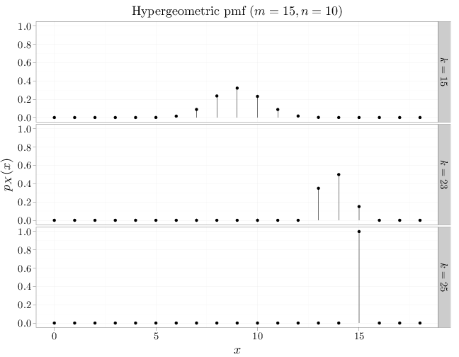
If the number of balls $m+n$ is much larger than $k$, the hypergeometric distribution converges to the binomial distribution (sampling without replacement is similar to sampling with replacement if the number of drawn balls is much smaller than the number of balls in the urn). This is illustrated by the first row in the figure above, which displays behavior similar to the corresponding binomial. The second and third rows show a strong deviation from the binomial model.