3.6. The Poisson Distribution

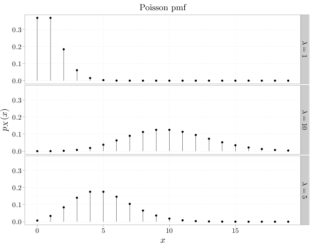
The Poisson RV, $X\sim \text{Pois}(\lambda)$, where $\lambda>0$, has the following pmf \begin{align*} p_X(x)=\begin{cases}\frac{\lambda^x e^{-\lambda}}{x!} & x\in\mathbb{N}\cup\{0\}\\ 0 & \text{otherwise} \end{cases}. \end{align*}

Using Taylor expansion (Section D.2) we ascertain that $P(X\in\Omega)=1$: \[\sum_{x=0}^{\infty}\frac{\lambda^x e^{-\lambda}}{x!}=e^{-\lambda} \sum_{x=0}^{\infty} \frac{\lambda^x}{x!}=e^{-\lambda}e^{\lambda}=1.\]

We denote the pmf of $X\sim\text{Bin}(n,\theta)$ by $\text{Bin}(x\,;n,\theta)$ and consider the case where $n\to\infty$, $\theta\to 0$ and $n\theta=\lambda\in (0,\infty)$. Using the geometric series formula (see Section D.2), we have \begin{align*} \log \text{Bin}(x=0\,;n,\theta) &=\log (1-\theta)^n=\log (1-\lambda/n)^n = n \log(1-\lambda/n) \\ &= -\lambda - \frac{\lambda^2}{2n}-\cdots, \end{align*} implying that \begin{align*} \text{Bin}(x=0\,;n,\theta) \approx \exp(-\lambda). \end{align*} Similarly, \begin{align*} \frac{\text{Bin}(x\,;n,\theta)}{\text{Bin}(x-1\,;n,\theta)} &= \frac{n-x+1}{n}\frac{\theta}{1-\theta} = \frac{\lambda-(x-1)\theta}{x(1-\theta)} \approx \frac{\lambda}{x}, \end{align*} implying that \begin{align*} \text{Bin}(x=1\,;n,\theta) &\approx \frac{\lambda}{x} \text{Bin}(x=0\,;n,\theta)\approx \frac{\lambda}{1}\exp(-\lambda) \\ \text{Bin}(x=2\,;n,\theta) &\approx \frac{\lambda}{x} \text{Bin}(x=1\,;n,\theta)\approx \frac{\lambda^2}{2\cdot 1}\exp(-\lambda). \end{align*} Using induction, we observe that the pmf of $\text{Pois}(\lambda)$ approximates the pmf of $\text{Bin}(n,\theta)$ when $n\to\infty$, $\theta\to 0$ and $n\theta=\lambda\in (0,\infty)$. In other words, the $\text{Pois}(\lambda)$ RV is the number of "successes" occurring in a very long sequence of independent Bernoulli experiments ($n\to\infty$), each having very small success probability $\theta\to 0$, and further assuming that $0 < n\theta < \infty$.

The approximation above explains why many naturally-occurring quantities follow a Poisson distribution. Examples of such quantities are (see (Feller, 1968) for more details):

1. the number of particles reaching a counter during the disintegration of radioactive material,
2. the number of bombs landing in different regions of London during the Second World War,
3. the number of bacteria found in different regions of a Petri dish,
4. the number of centenarians (people over the age of 100) dying each year,
5. the number of cars arriving at an intersection during a particular time interval, and
6. the number of phone calls arriving at a switchboard during a particular time interval.

Using Taylor expansion (see Section D.2), we derive the mgf of the Poisson RV \begin{align*} m(t) =\sum_{k=0}^{\infty} e^{tk} \frac{\lambda^k e^{-\lambda}}{k!} =e^{-\lambda}\sum_{k=0}^{\infty} \frac{(e^{t}\lambda)^k }{k!} = e^{\lambda e^t-\lambda}, \end{align*} which leads to the following expectation and variance expressions: \begin{align*} \E(X) &= m'(0) = e^{\lambda e^t-\lambda}\lambda e^t\Big|_{t=0}=\lambda\\ \Var(X)& = \E(X^2)-(\E(X))^2 = m''(0)-\lambda^2 = \left(e^{\lambda e^t-\lambda}\lambda^2 (e^t)^2 +e^{\lambda e^t-\lambda}\lambda e^t \right)\Big|_{t=0} - \lambda^2 \\ &= \lambda. \end{align*} Proposition 4.8.1 states that the mgf of a sum of independent RVs is a product of the corresponding mgfs. Since the product of multiple Poisson mgfs with parameters $\lambda_i$ is also a Poisson mgf with parameter $\sum_i \lambda_i$, we have the following result: if $Z_i\sim \text{Pois}(\lambda_i)$, $i=1,\ldots,n$, are independent Poisson RVs then \[\sum_{i=1}^n Z_i \sim \text{Pois} \left(\sum_{i=1}^n \lambda_i\right). \]

x = 0:19
D = stack(list(`$\\lambda=1$` = dpois(x, 1), `$\\lambda=5$` = dpois(x,
    5), `$\\lambda=10$` = dpois(x, 10)))
names(D) = c("mass", "lambda")
D$x = x
qplot(x, mass, data = D, main = "Poisson pmf", geom = "point",
    stat = "identity", xlab = "$x$", ylab = "$p_X(x)$",
    facets = lambda ~ .) + geom_linerange(aes(x = x,
    ymin = 0, ymax = mass))