4.4. Functions of a Random Vector
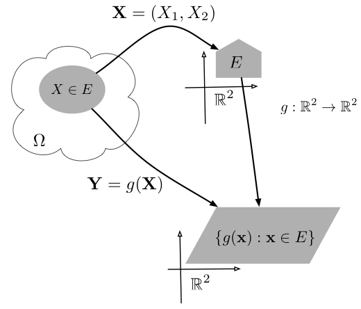
Recall that when $X$ is a random variable and $g:\mathbb{R}\to\mathbb{R}$ is a real valued function then $g(X)$ is also a random variable and its cdf, pdf or pmf are directly related to the corresponding functions of $X$ (Chapter 2). The same holds for a random vector. Specifically, for a random vector $\bb{X}=(X_1, \ldots, X_n)$ and \[g=(g_1, \ldots, g_k) : \R^n\to\R^k, \qquad g_i:\mathbb{R}^n \to \mathbb{R}, \quad i=1,\ldots,k,\] we have a new $k$-dimensional random vector $\bb{Y}=g(\bb{X})$ with \[Y_i=g_i(X_1,\ldots,X_n),\quad i=1,\ldots,k.\] Figure 4.4.1 illustrates this concept.
As in the case of random variables, we consider several techniques for relating the cdf, pmf, or pdf of $g(\bb X)$ to that of $\bb X$.
- The first technique is to compute the cdf $F_{\bb{Y}}(\bb{y})$, for all $\bb{y}\in\mathbb{R}^k$. When $k=1$, $\bb{Y}=Y=g(X_1,\ldots,X_n)$ and \begin{align*} F_Y(y)=\P(g(X_1,\ldots,X_n)\leq y) =\begin{cases} \int_{\bb{x}:g(\bb{x})\leq y} f_{\bb{X}}(\bb{x})d\bb{x} & \bb{X} \text{ is continuous }\\ \sum_{\bb{x}:g(\bb{x})\leq y} p_{\bb{X}}(\bb{x}) & \bb{X} \text{ is discrete }\\ \end{cases}. \end{align*} When $k > 2$, \begin{align*} F_{Y_1,\ldots,Y_k}(y_1,\ldots, y_k) &= \P(g_1(\bb{X})\leq y_1,\ldots,g_k(\bb{X})\leq y_1) \\ &=\begin{cases}\int_A f_{\bb{X}}(\bb{x}) \, d\bb{x} & \bb{X} \text{ is continuous}\\ \sum_{\bb{x}\in A} p_{\bb{X}}(\bb{x}) & \bb{X} \text{ is discrete} \end{cases} \end{align*} where \[A=\{\bb{x}\in\mathbb{R}^n: g_j(\bb{x})\leq y_j \text{ for } j=1,\ldots,k\}.\]
- If $\bb{Y}$ is discrete we can find its pmf by \begin{align*} p_{\bb{Y}}(y_1,\ldots,y_k)&=\P(g_1(\bb{X})= y_1,\ldots, g_k(\bb{X})= y_k) \\&=\begin{cases}\int_A f_{\bb{X}}(\bb{x}) \, d\bb{x} & \bb{X} \text{ is continuous}\\ \sum_{\bb{x}\in A} p_{\bb{X}}(\bb{x}) & \bb{X} \text{ is discrete} \end{cases} \end{align*} where \[A=\{\bb{x}\in\mathbb{R}^n: g_j(\bb{x})= y_j \text{ for all } j=1,\ldots,k\}.\] Note that if $g$ is one-to-one the set $A$ consists of a single element.
-
If $\bb{Y}$ is continuous we can obtain the pdf $f_{\bb{Y}}$
by differentiating the joint cdf (if it is available)
\[f_{\bb{Y}}(\bb{y})=\frac{\partial^k}{\partial y_1\cdots \partial y_k } F_{\bb{Y}}(\bb{y})\]
or using the change of variable technique assuming that $k=n$ (see below).
Proposition 4.4.1. For an $n$-dimensional continuous random vector $\bb{X}$ and $\bb{Y}=g(\bb{X})$ with an invertible and differentiable $g:\R^n\to\R^n$ (in the range of $\bb{X}$), \[ f_{\bb{Y}}(\bb{y}) \cdot |\det J(g^{-1}(\bb{y}))| = f_{\bb{X}}(g^{-1}(\bb{y}))\] where $J(g^{-1}(\bb{y}))$ is the Jacobian matrix at $\bb{x}=g^{-1}(\bb{y})$: \begin{align*} J(\bb{x})=\begin{pmatrix} \frac{\partial g_1}{\partial x_1}(\bb{x})& \cdots & \frac{\partial g_1}{\partial x_n}(\bb{x})\\ \vdots & \vdots & \vdots\\ \frac{\partial g_n}{\partial x_1}(\bb{x})& \cdots & \frac{\partial g_n}{\partial x_n}(\bb{x})\\ \end{pmatrix}. \end{align*}Proof. See Proposition F.6.3.
- The third technique uses the moment generating function. See the corresponding technique in Chapter 2 and the generalization of the moment generating function to random vectors at the end of this chapter.
The following example illustrates the second method above in the important special case of an invertible linear transformation (see Chapter C).
The example above leads to a general technique for finding the pdf or pmf of a sum of independent random variables. This is explored in the example below. Proposition 4.4.3 shows how to obtain the same result using the convolution operator.
The example below illustrates the second method of finding the distribution of $g(\bb X)$ in the case of a non-linear transformation $g$.
The parenthesis are often omitted resulting in the notation $f*g$.
The convolution's associativity justifies leaving out the parenthesis, for example we write $(f*g*h)(t)$ instead of $(f*(g*h))(t)$.