6.4. One Dimensional Random Walk

Thus far, we examined in detail two simple processes: the sinusoidal process where every random variable is a function of any other random variable and the iid process where every random variable is independent of any other random variable. We consider in this section the random walk process, an RP that is neither independent nor completely dependent. In the next chapter, we will see in detail four additional RPs: the Poisson process, the Markov chain, the Gaussian process, and the Dirichlet process.

Recall from Example 6.3.4 the RP $\mathcal{Y}=\{Y_t: t\in\mathbb{N}\}$ where $Y_t$ are iid random variables taking value 1 with probability $\theta$ and $-1$ with probability $1-\theta$. The random walk process is the discrete-time discrete-state random process $\mathcal{Z}=\{Z_t:t=1,2,\ldots\}$ where \[Z_t=\sum_{n=1}^t Y_n.\] Note that $\mathcal{Z}$ is neither iid nor completely dependent, and it has independent increments; for example, $Z_5-Z_3=Y_4+Y_5$ and $Z_9-Z_7=Y_8+Y_9$ are independent RVs, as they are sums of iid RVs.

The term random walk comes from the following interpretation. Consider a walker who chooses each step at random. The walker chooses whether to walk forward with probability $\theta$ or backward with probability $1-\theta$. The position of the walk at time $t$ is precisely $Z_t$ (assuming the walker starts from 0). An alternative interpretation is related to gambles that win one dollar with probability $\theta$ and lose one dollar with probability $1-\theta$. The RV $Z_t$ measures the total profit or losses of a persistent gambler at time $t$, assuming the gambler can continue gambling forever (more realistically a gambler with a fixed fortune will not be able to continue gambling after losing all of the money).

The moment functions for $\mathcal{Z}$ are the following functions: for all $t,t_1,t_2\in\mathbb{N}$ \begin{align*} m(t) &= \E\left(\sum_{i=1}^t Y_i\right) = \sum_{i=1}^t \E(Y_i) =t(2\theta-1)\\ v(t) &= \Var\left(\sum_{i=1}^t Y_i\right) = t \Var(Y_1)=4t\theta(1-\theta)\\ C(t_1,t_2) &= \E\left(\left(\sum_{i=1}^{t_1} (Y_i-\E(Y_1))\right) \left(\sum_{j=1}^{t_2} (Y_j-\E(Y_1))\right)\right)\\ &= \E\left(\sum_{i=1}^{t_1}\sum_{j=1}^{t_2} (Y_i-\E(Y_1))(Y_j-\E(Y_1))\right)\\ &=\sum_{i=1}^{t_1}\sum_{i=1}^{t_2} \E((Y_i-\E(Y_1))(Y_j-\E(Y_1))) = \sum_{i=1}^{t_1}\sum_{i=1}^{t_2} \delta_{t_1,t_2}4\theta(1-\theta) \\ &= \min(t_1,t_2) 4\theta(1-\theta)\\ \rho(t_1,t_2) &= \frac{C(t_1,t_2)}{\sqrt{v(t_1)v(t_2)}} = \frac{\min(t_1,t_2)}{\sqrt{t_1t_2}}. \end{align*}

The expectation function $m$ increases linearly if $\theta > 0.5$, decreases linearly if $\theta < 0.5$ and is 0 if $\theta=0.5$. This is in agreement with our intuition that a sequence of gambles biased towards winning will tend to continually increase the fortune as $t$ increases, and vice verse for gambles biased towards losing. The variance function linearly increases as $t\to\infty$.

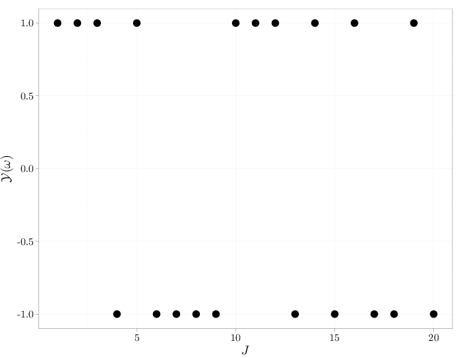
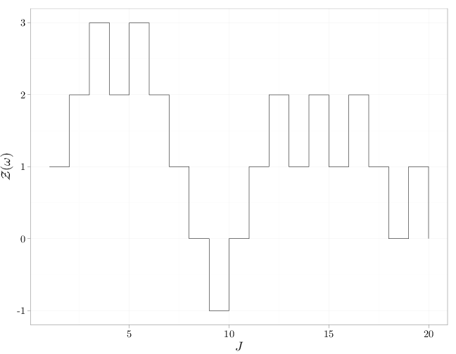
The R code below graphs a realization of $\mathcal{Y}=\{Y_t:t\in\mathbb{N}\}$ followed by a corresponding realization of $\mathcal{Z}$ for $\theta=0.6$ for $t\leq 20$.

J = 1:20
X = rbinom(n = 20, size = 1, prob = 0.6)
Y = 2 * X - 1
qplot(x = J, y = Y, geom = "point", size = I(5), xlab = "$J$",
    ylab = "$\\mathcal{Y}(\\omega)$")

qplot(x = J, y = cumsum(Y), geom = "step", xlab = "$J$",
    ylab = "$\\mathcal{Z}(\\omega)$")

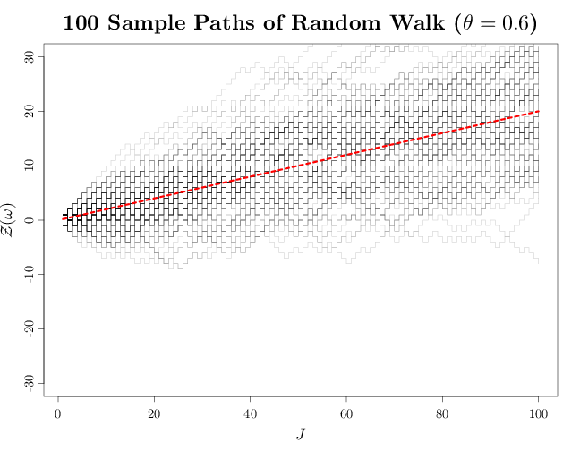
The R code below graphs multiple sample paths sampled from $\mathcal{Z}$, superimposed with the expectation function $m(t)$ for the case $\theta=0.6$. The graph uses transparency to show high or low density of sample paths where multiple sample paths overlap. In this case, the gambles are biased towards winning, and the gambler's fortune will tend to increase in most cases (though a long unfortunate run is still possible). Note how the process tends to move linearly upwards as $t$ increases, which is in agreement with the above derivation for $m(t)$. The increase in the variability of the fortune as $t$ increases is in agreement with the linear increase of $v(t)$ derived above.

par(cex.main = 2, cex.axis = 1.2, cex.lab = 1.5)
plot(c(1, 100), c(-30, 30), type = "n", xlab = "$J$",
    ylab = "$\\mathcal{Z}(\\omega)$")
Zn = vector()
for (i in 1:100) {
    X = rbinom(n = 100, size = 1, prob = 0.6)
    Z = cumsum(2 * X - 1)
    lines(1:100, c(Z), type = "s", col = rgb(0, 0,
        0, alpha = 0.2))
    Zn[i] = Z[100]
}
curve(x * (2 * 0.6 - 1), add = TRUE, col = rgb(1, 0,
    0), lwd = 5, lty = 2)
title("100 Sample Paths of Random Walk ($\\theta=0.6$)")

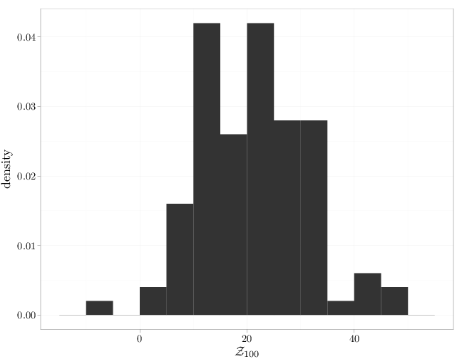
The R code below graphs the histogram of the random walk (or gambler's fortunes) at $t=100$ based on the 100 sample paths computed above. This represents the distribution of $Z_{100}$. The average fortune seems to be around 20, which is precisely the value of $m(100)$ for $\theta=0.6$. The shape of the histogram is in agreement with a sample from the binomial distribution of $Z_n$ (see Exercise 3 at the end of this chapter).

qplot(Zn, ..density.., binwidth = 5, xlab = "$\\mathcal{Z}_{100}$",
    geom = "histogram")

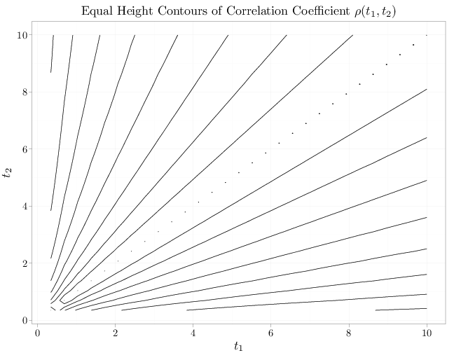
The R code below graphs the equal height contours of the correlation coefficient function, as a function of $t_1$, $t_2$, for the case of $\theta=0.6$. We have $\rho(t_1,t_2)=1$ for $t_1=t_2$ indicating perfect correlation. As $|t_1-t_2|$ increases, the correlation coefficient decays in agreement with our intuition that the random walk process at two disparate time points is not highly correlated.

x = seq(0, 10, length.out = 30)
R = expand.grid(x, x)
names(R) = c("t1", "t2")
R$covariance = pmin(R$t1, R$t2)/(sqrt(R$t1 * R$t2))
P = ggplot(R, aes(x = t1, y = t2, z = covariance)) +
    xlab("$t_1$") + ylab("$t_2$") + stat_contour()
P + opts(title = "Equal Height Contours of Correlation Coefficient $\\rho(t_1,t_2)$")