Probability
The Analysis of Data, volume 1
Random Vectors: Basic Definitions
$
\def\P{\mathsf{\sf P}}
\def\E{\mathsf{\sf E}}
\def\Var{\mathsf{\sf Var}}
\def\Cov{\mathsf{\sf Cov}}
\def\std{\mathsf{\sf std}}
\def\Cor{\mathsf{\sf Cor}}
\def\R{\mathbb{R}}
\def\c{\,|\,}
\def\bb{\boldsymbol}
\def\diag{\mathsf{\sf diag}}
\def\defeq{\stackrel{\tiny\text{def}}{=}}
$
4.1. Basic Definitions
In the previous chapters we considered random variables $X:\Omega\to \R$ and the probabilities associated with them $\P(X\in A)$. Whenever we discussed multiple random variable $X,Y$ we assumed independence: $\P(X\in A, Y\in B)=\P(X\in A)\P(Y\in B)$. In this chapter we extend our discussion to multiple (potentially) dependent random variables. Our exposition is general, and applies to $n$ random variables, but it is useful to keep in mind the intuitive $n=2$ case. We continue in this chapter our approach of considering random vectors that are either discrete or continuous. This allows us to avoid using measure theory in most of the proofs.
Definition 4.1.1.
A random vector $\bb{X}=(X_1,\ldots,X_n)$ is a collection of $n$ random variables $X_i:\Omega\to\R$ that together may be considered a mapping $\bb{X}:\Omega\to\mathbb{R}^n$. We denote
\begin{align*}
\{\bb{X}\in E\} &\defeq \{\omega\in\Omega: (X_1(\omega),\ldots,X_n(\omega)) \in E\}, \qquad E\subset \mathbb{R}^n,\\
\P(\bb{X}\in E) &= \P(\{\omega\in\Omega: \bb{X}(\omega)=(X_1(\omega),\ldots,X_n(\omega))\in E\}).
\end{align*}
Figure 4.1.1 illustrates the definition above. Note that we denote random vectors in bold-face and its components using subscripts, for example $\bb{X}=(X_1,\ldots,X_n)$. This mirrors our notation of vectors in $\R^n$ using lower-case bold-face letters, for example $\bb{x}=(x_1,\ldots,x_n)\in\R^n$.
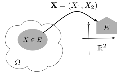
Figure 4.1.1: A random vector $\bb{X}=(X_1,X_2)$ is a mapping from $\Omega$ to $\mathbb{R}^2$. The set $\{\bb{X}\in E\}$ is a subset of $\Omega$ corresponding to all $\omega\in\Omega$ that are mapped to $E$.
Definition 4.1.1.
If a set $E\subset \mathbb{R}^n$ is of the form $E=\{\bb{x}\in\mathbb{R}^n: x_1\in S_1,\ldots,x_n\in S_n \}$, we call it a product set and denote it as $E=S_1\times\cdots \times S_n$.
Figure 4.1.2 illustrates the definition above.
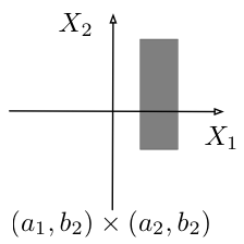
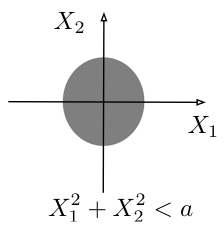
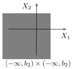
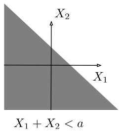
Figure 4.1.2: Two product sets (top) and two non-product sets (bottom) for $\bb{X}=(X_1,X_2)$.
Definition 4.1.1.
Two RVs, $X_1,X_2$, are independent if for all product sets, $S_1\times S_2$
\[ \P((X_1,X_2)\in S_1\times S_2) = \P(X_1\in S_1)\P(X_2\in S_2).\]
The components of a random vector are pairwise independent if every pair of components is independent. The components of a random vector $\bb{X}=(X_1,\ldots,X_n)$ are independent if for all product sets $S_1\times\cdots\times S_n$,
\[ \P(\bb{X}\in S_1\times \cdots\times S_n) = \P(X_1\in S_1) \cdots \P(X_n \in S_n).\]
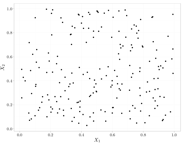
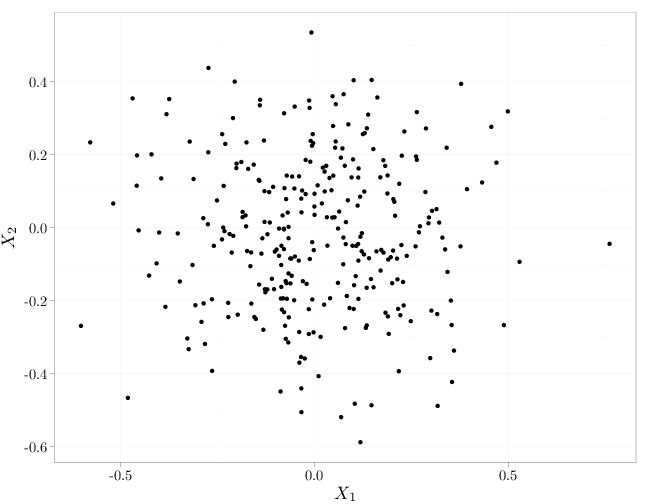
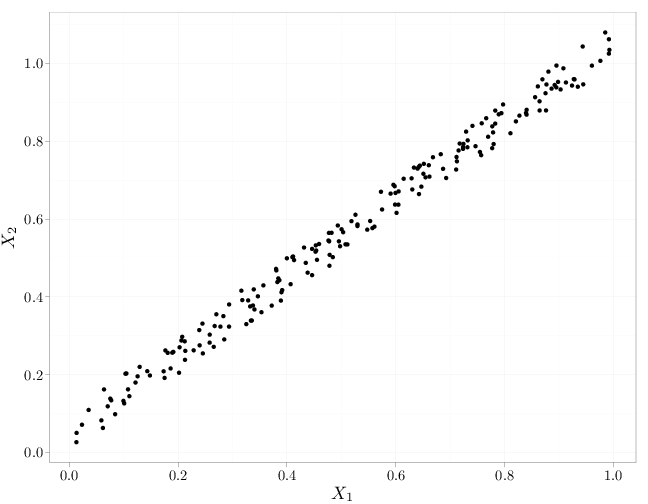
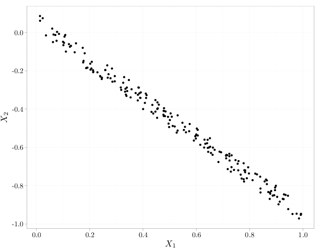
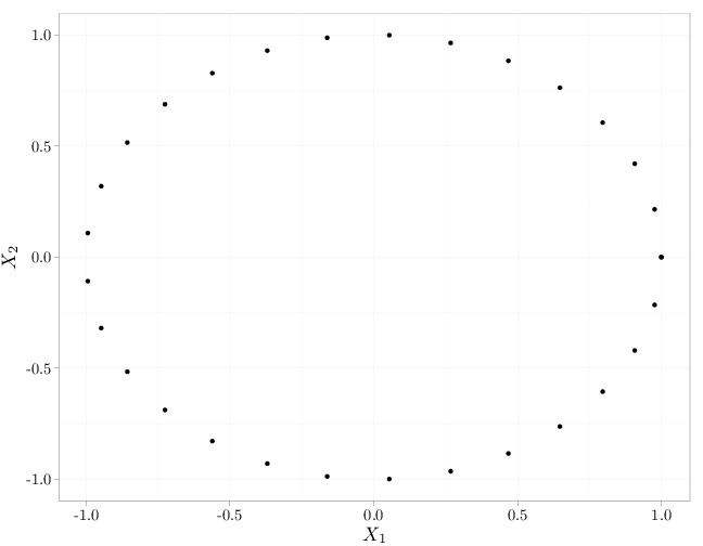
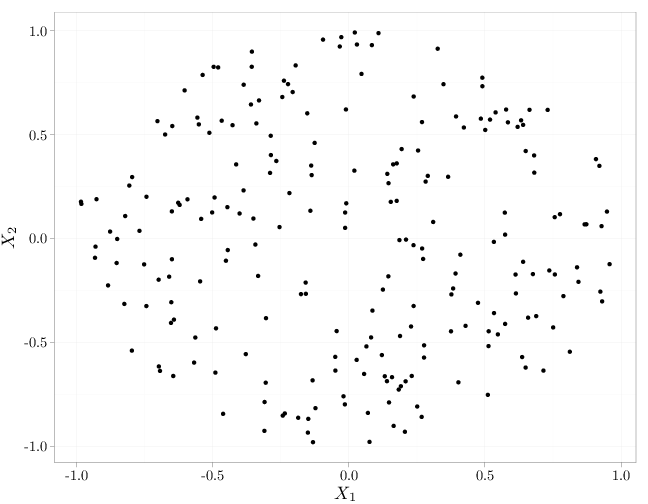
As in the case of independence of events (Definition 1.5.2), mutual independence implies pairwise independence but not necessarily vice verse. The R code below graphs samples from several independent and dependent random vectors $(X_1,X_2)$. The cases in the top row exhibit independence (uniform distribution in the unit square and spherical symmetric distribution with more samples falling closer to the origin). The middle row and bottom row exhibit a lack of independence (knowing the value of $X_2$ influences the probability of $X_1$: $\P(X_1|X_2)\neq \P(X_1)$. The top and bottom rows exhibit zero covariance while the middle row exhibits positive covariance (left) and negative covariance (right).
X = runif(200)
Y = runif(200)
W = rnorm(300, sd = 0.2)
Z = rnorm(300, sd = 0.2)
Q = runif(300) * 2 - 1
P = runif(300) * 2 - 1
qplot(X, Y, xlab = "$X_1$", ylab = "$X_2$")
qplot(W, Z, xlab = "$X_1$", ylab = "$X_2$")
qplot(X, X + runif(200)/10, xlab = "$X_1$", ylab = "$X_2$")
qplot(X, -X + runif(200)/10, xlab = "$X_1$", ylab = "$X_2$")
qplot(cos(seq(0, 2 * pi, length = 30)), sin(seq(0,
    2 * pi, length = 30)), xlab = "$X_1$", ylab = "$X_2$")
qplot(Q[(Q^2 + P^2) < 1], P[(Q^2 + P^2) < 1], xlab = "$X_1$",
    ylab = "$X_2$")
Example 4.1.1.
In a random experiment describing drawing a phone number from a phone book, the sample space $\Omega$ is the collection of phone numbers and an outcome $\omega\in\Omega$ corresponds to a specific phone number. Let $X_1, X_2, X_3:\Omega\to\mathbb{R}$ be the weight, height, and IQ of the phone number's owner. The event
\[\{X_1 \in (a_1,b_1)\}=\{\omega\in\Omega:X_1(\omega)\in(a_1,b_1)\}\] corresponds to ``the weight of the selected phone number's owner lies in the range $(a_1,b_1)$''. The event $(X_1,X_2) \in (a_1,b_1)\times (a_2,b_2)$ corresponds to ``the weight is in the range $(a_1,b_1)$ and the height is in the range $(a_2, b_2)$''. The set $(a_1,b_1)\times (a_2,b_2)$ is a product set, but since we do not expect height and weight to be independent RVs, we normally have
\[\P((X_1,X_2) \in (a_1,b_1)\times (a_2,b_2))\neq \P(X_1\in(a_1,b_1))\P(X_2\in(a_2,b_2)).\]
The set $(a_2,b_2)\times (a_3,b_3)$ is also a product event, and assuming that height and IQ are independent, we have
\[\P((X_2,X_3) \in (a_2,b_3)\times (a_3,b_3))= \P(X_2\in(a_2,b_2))\P(X_3\in(a_3,b_3)).\]
Two examples of non-product sets are $X_2/X_1^2 \leq a$ (body-mass index less than $a$) and $X_1\leq X_2+a$.
A random vector $\bb X$ with corresponding $\Omega, \P$ defines a new distribution $\P'$ on $\Omega'=\mathbb{R}^n$:
\[\P'(E)=\P(\bb{X}\in E).\]
It is straightforward to verify that $\P'$ satisfies the three probability axioms.
In many cases the probability space $(\R^n,\P')$ is conceptually simpler than $(\Omega,\P)$.
Definition 4.1.2.
In the dice-throwing experiment (Example 1.3.1), for $X_1(a,b)=a+b$ (an RV measuring the sum of the outcomes of two dice) and $X_2(a,b)=a-b$ (an RV measuring the difference of the outcomes of the two dice) we have
\begin{align*}
\P(X_1=2,X_2=2)&=\P(X_1\in\{2\},X_2\in\{2\})=\P(\emptyset)=0\\
\P(X_1=6,X_2=2)&=\P(\{(4,2)\})=1/36\\
\P(X_1 > 4,X_2 < 0) &=\P(\{(1,4),(1,5),(1,6),(2,3),(2,4),(2,5), \\
& \qquad (2,6),(3,4),(3,5),(3,6),(4,5),(4,6),(5,6)\}) = \frac{13}{36}\\
\P(X_1 > 4) &= 1-\P(\{(1,1),(1,2),(2,1),(1,3),(3,1),(2,2)\})=30/36\\
\P(X_2 < 0) &= 15/36.
\end{align*}
Since $\P(X_1 > 4,X_2 < 0)\neq \P(X_1 > 4)\P(X_2 < 0)$, $X_1,X_2$ are not independent.