8.9. Central Limit Theorem
The central limit theorem shows that the distribution of $n^{-1}\sum_{i=1}^n \bb{X}^{(i)}$ for large $n$ is Gaussian centered around $\mu=\E(\bb X)$ with variance $\Sigma/n$. Thus, not only can we say that $n^{-1}\sum_{i=1}^n \bb{X}^{(i)}$ is close to $\bb \mu$ (as the law of large numbers implies), we can say that its distribution is a bell shaped curve centered at $\bb \mu$ whose variance decays linearly with $n$.
We denote by $\tilde \phi$ the characteristic functions of ${\bb X}^{(k)}-\E({\bb X}^{(k)})$, $k\in\mathbb{N}$ (${\bb X}^{(k)}$ are iid and so they have the same characteristic function). Since $\tilde \phi(\bb 0)=1$, $\nabla \tilde \phi(\bb 0)=\bb 0$, and $\lim_{\bb\epsilon\to \bb 0}\nabla^2\tilde \phi(\bb\epsilon)=\Sigma$, we have \begin{align*} \lim_{n\to\infty} \phi_{\sqrt{n}(\sum_{k=1}^n {\bb X}^{(k)}/n-\bb\mu)} (\bb t) &= \lim_{n\to\infty} \phi_{(\sum_{k=1}^n {\bb X}^{(k)}/n-\bb\mu)} (\bb t/\sqrt{n})\\ &= (\tilde\phi(\bb t/\sqrt{n}))^n\\ &= \lim_{n\to\infty} \left(1+ \frac{1}{n}{\bb t}^{\top}\int_0^1\int_0^1 z \nabla^2 \phi(zw\bb t/\sqrt{n})\,dzdw\,\bb t \right)^n\\ &= \left(\lim_{n\to\infty} \frac{1}{n}{\bb t}^{\top}\int_0^1\int_0^1 z \nabla^2 \phi(zw\bb t/\sqrt{n})\,dzdw\,\bb t \right)^n\\ &=\exp(-{\bb t}^{\top}\Sigma\bb t/2)\\ &=\phi_{N(\bb 0,\bb \Sigma)}. \end{align*} The second to last equality follows from Proposition D.2.2, and the last equality follows from Proposition 8.7.2.
We make the following comments concerning the central limit theorem (CLT):
- Statisticians generally agree as a rule of thumb that the approximation in the CLT is accurate when $n > 30$ and $d=1$. However, the CLT approximation can also be effectively used in many cases where $n < 30$ or $d > 1$.
- Since a linear combination of a multivariate Gaussian random vector is a multivariate Gaussian random vector, we have the following implications: \begin{align*} \sqrt{n}\left(\frac{1}{n}\sum_{i=1}^n {\bb X}^{(i)}-\bb \mu\right)\sim N(\bb 0,\Sigma)\quad &\Rightarrow \quad \frac{1}{n}\sum_{i=1}^n {\bb X}^{(i)}-\bb \mu\sim N(\bb 0,n^{-1}\Sigma)\\ \quad &\Rightarrow \quad \frac{1}{n}\sum_{i=1}^n {\bb X}^{(i)} \sim N(\bb \mu,n^{-1}\Sigma)\\ \quad &\Rightarrow \quad \sum_{i=1}^n {\bb X}^{(i)} \sim N(n\bb \mu,n \Sigma). \end{align*} As a result, we can say that intuitively, $\frac{1}{n}\sum_{i=1}^n {\bb X}^{(i)}$ has a distribution that is approximately $N(\bb \mu,n^{-1}\Sigma)$ for large $n$ i.e., it is approximately a Gaussian centered at the expectation and whose variance is decaying linearly with $n$. Similarly, intuitively, the distribution of $\sum_{i=1}^n {\bb X}^{(i)}$ for large $n$ is approximately $N(n\bb \mu,n^2\Sigma/n) = N(n\bb \mu,n\Sigma)$.
- The CLT is very surprising. It states that if we are looking for a distribution of a random vector $\bb Y$ that is a sum or average of many other iid random vectors ${\bb X}^{(i)}$, $i=1,\ldots,n$, the distribution of $\bb Y$ will be close to normal regardless of the distribution of the original ${\bb X}^{(i)}$. This explains the fact that many quantities in the real world appear to have a Gaussian distribution or close to it. Examples include physical measurements like height and weight (they may be the result of a sum of many independent RVs expressing genetic makeup), atmospheric interference (sum of many small interference on a molecular scale), and movement of securities prices in finance (sum of many buy or sell orders).
- The condition of iid in the CLT above may be relaxed. More general results state that a sum of many independent (but not identically distributed) RVs is Gaussian under relatively weak conditions. Even the independence assumption may be relaxed as long as it is not the case that every example depends on most of the other examples.
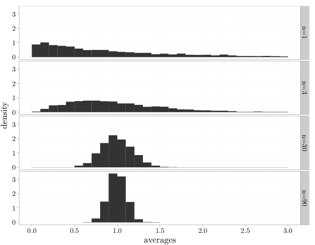
The code below displays the histograms of averages of $n=1, 3, 30, 90$ iid samples from a $\text{Exp}(\lambda)$ distribution (with $\mu=1$). Note how, as $n$ increases, the averages tend to concentrate increasingly around the average 1, which reflects the weak law of large numbers. The CLT is evident in that the histogram for large $n$ resembles a bell-shaped curve centered at the expectation. Note also how the histogram width decreases from 30 to 90 as $n$ increases according to $\Sigma/n$, in agreement with the decay of the asymptotic variance.
iter = 2000
avg0 <- avg1 <- avg2 <- avg3 <- rep(0, iter)
for (i in 1:iter) {
    S = rexp(90)  # sample from exp(1) distribution
    avg0[i] = S[1]
    avg1[i] = mean(S[1:3])
    avg2[i] = mean(S[1:30])
    avg3[i] = mean(S[1:90])
}
SR = stack(list(`n=1` = avg0, `n=3` = avg1, `n=30` = avg2,
    `n=90` = avg3))
names(SR) = c("averages", "n")
ggplot(SR, aes(x = averages, y = ..density..)) + facet_grid(n ~
    .) + geom_histogram() + scale_x_continuous(limits = c(0,
    3))